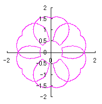
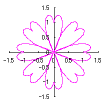
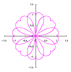
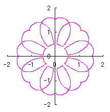
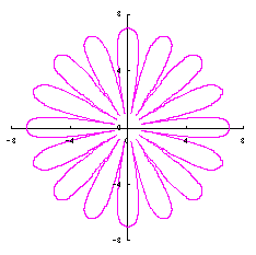
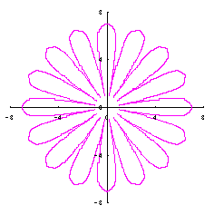
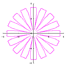
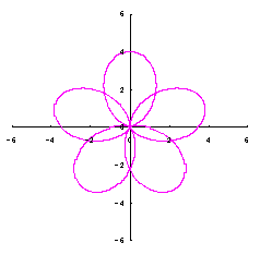
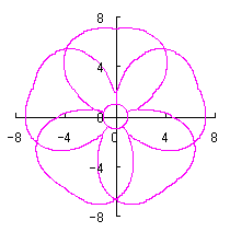
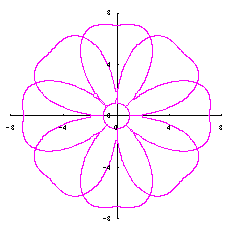
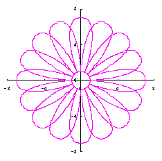
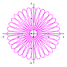
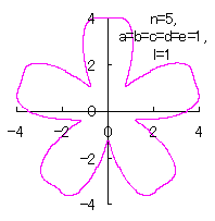
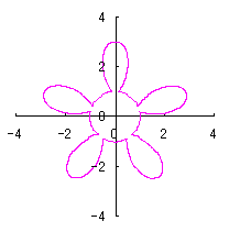
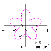
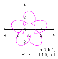
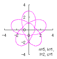
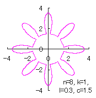
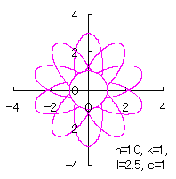
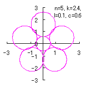
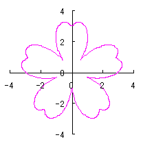
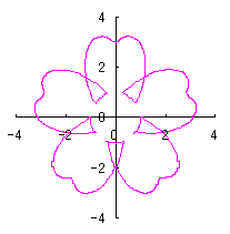
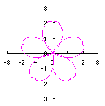
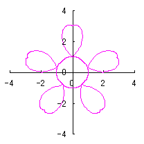
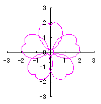
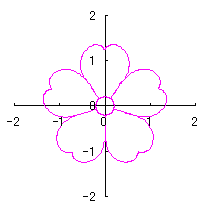
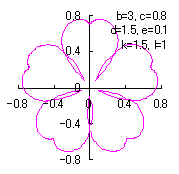
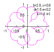
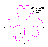
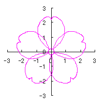
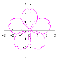
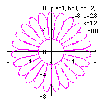
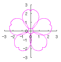
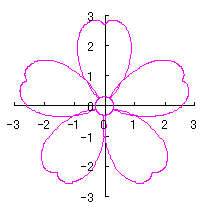
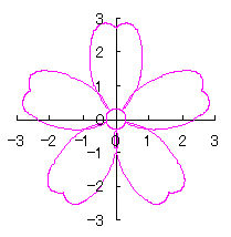
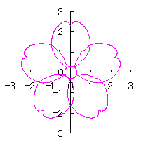
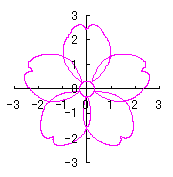
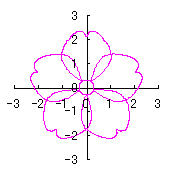
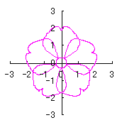
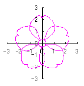
TDCC Laboratory

   HOME JAPANESE                                        

Flower Graphics

Nobuo YAMAMOTO

You can copy and use all the figures in this page freely.


1.  Preface

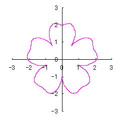
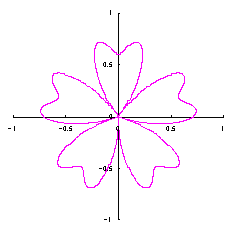
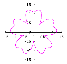
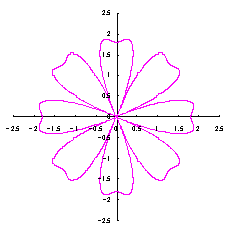
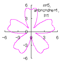
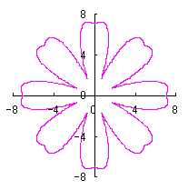
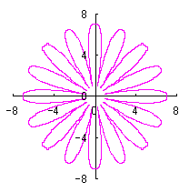
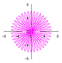
     We try to produce shape of flower by calculation with the use of computer as an application of "heart curves II" treated in the other page of this home page.    According to two kinds of methods written in the page of "heart curves II", these two methods will be followed also in this page.


2.  Method 1
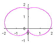
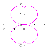
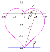
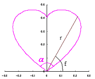
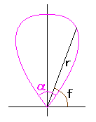
Fig.1b  Heart curve 1
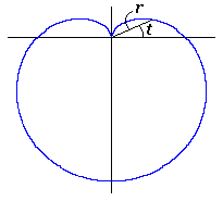
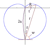
Fig.1a  The original Cardioid

     Method 1 is to make a heart curve from a Cardioid by forming an angle on its bottom simply, where the heart curve will be used as a petal of a flower,


2.1    In the case of no change in the length and width of heart curve to be used as a petal of flower

     The original Cardioid is shown in Fig,1a, and the heart curve, which is produced from this original Cardioid by the method 1 as described in the page of "heart curves II", is shown in Fig.1b.    We intend to form a shape of flower by arranging heart curves around a center circle as petals of a flower.
    The equations obtained in the page of "heart curves II" and used also in this page are the following three ones;

          ,                      (1)
where .

          ,                      (2)
where .

          .                      (3)

    We will arrange such the obtained heart curves around a center circle as petals of a flower.    If numbers of petals are arranged, we assume that the bottom angle of a heart curve is taken as the angle of going around a flower divided by as given in the following equation;
          .                      (4)

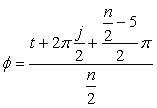
    When the number is assigned to each of petals, the phase angle of -th number's of petal is expressed in the following equation into which the angle is added to .

          .                      (5)

    Thus, numbers of petals around a center circle are described above,    If the radius of its surrounded cicle by petals is , a whole flower is expressed in the following two equations in the orthogonal (x, y) coordinates.
          .                      (6)
          .                      (7)

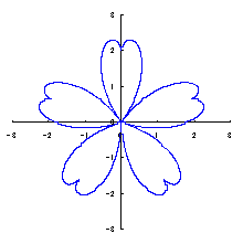
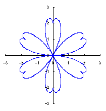
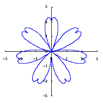
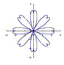
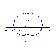
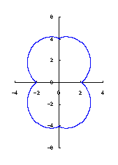
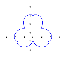
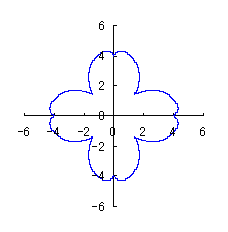
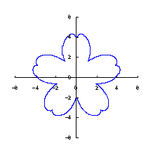
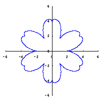
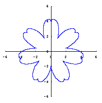
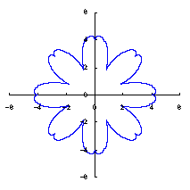
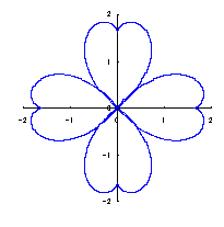
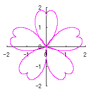
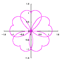
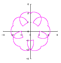
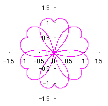
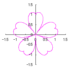
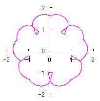
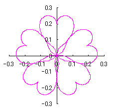
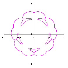
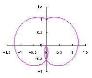
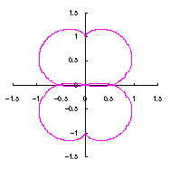
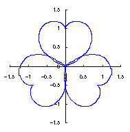
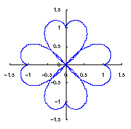
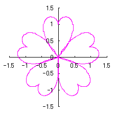
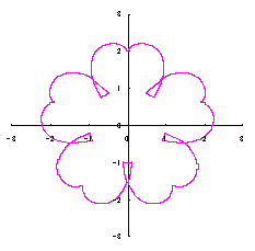
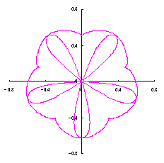
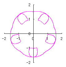
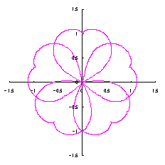
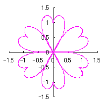
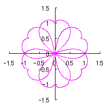
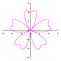
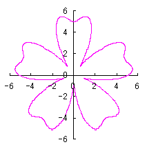
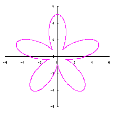
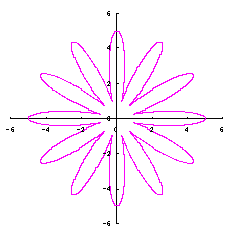
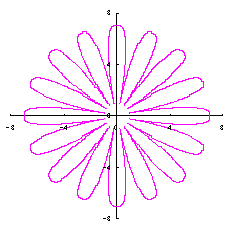
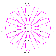
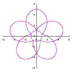
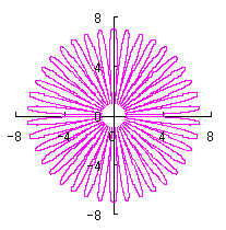
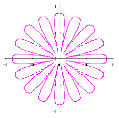
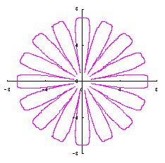
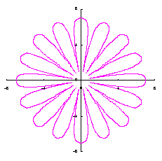
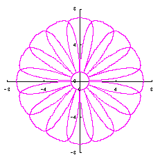
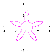
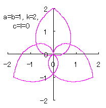
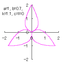
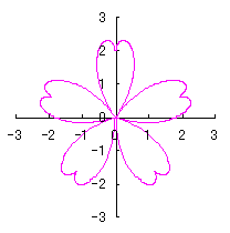
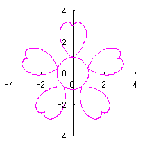
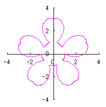
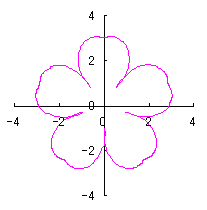
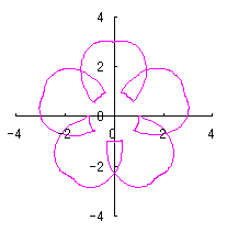
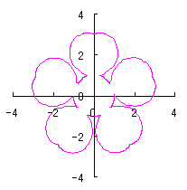
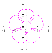
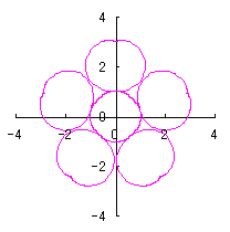
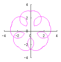
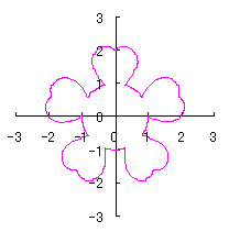
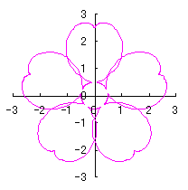
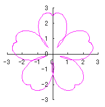
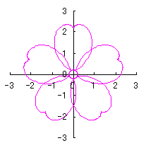
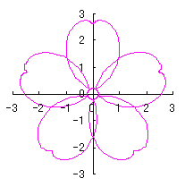
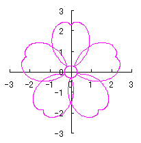
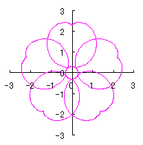
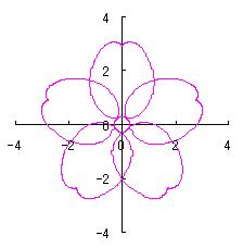
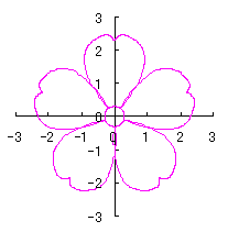
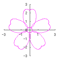
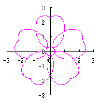
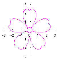
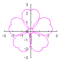
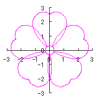
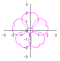
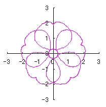
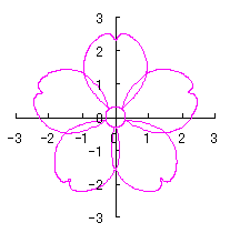
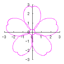
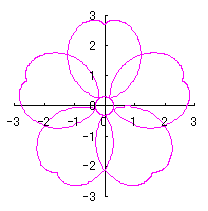
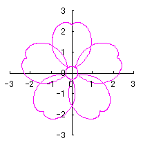
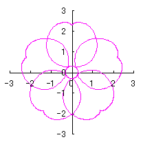
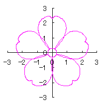
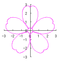
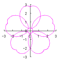
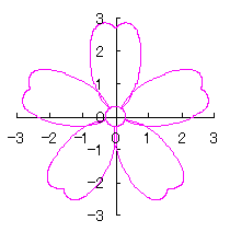
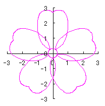
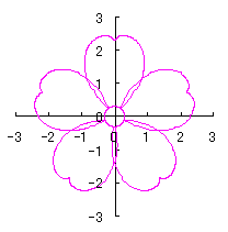
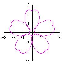
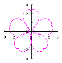
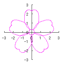
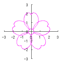
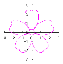
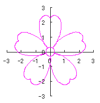
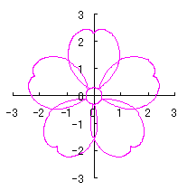
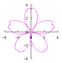
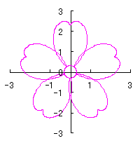
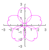
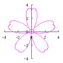
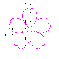
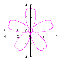
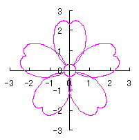
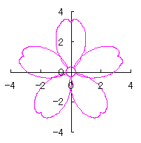
    By calculating Eqs.(1), (2), (4), (5), (6) and (7), the (x, y) coordinate data of shape of a flower are obtained.    Examples of such obtained shape of flower in the case of are shown in Figs.2 to 16 where decides only the size and does not relate to the shape.

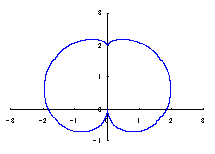
Fig.2  n=1, c=0
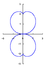
Fig.3  n=2, c=0
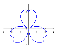
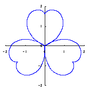
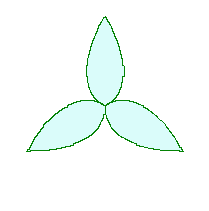
Fig.4  n=3, c=0
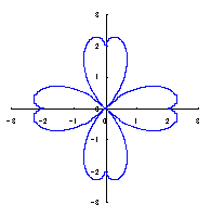
Fig.5  n=4, c=0

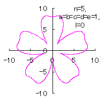
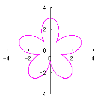
Fig.6  n=5, c=0
Fig.7  n=6, c=0
Fig.8  n=7, c=0
Fig.9  n=8, c=0

Fig.10  n=1, c=2
Fig.11  n=2, c=2
Fig.12  n=3, c=2
Fig.13  n=4, c=2

Fig.14  n=8, c=2
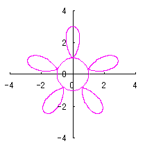
Fig.15  n=5, c=2
Fig.16  n=6, c=2
Fig.17  n=7, c=2

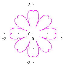
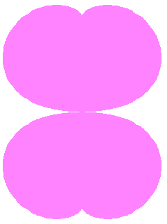
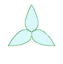
     When the above figures are painted, the following ones are drawn.    If clicked, an expanded line drawing appears.


Fig.2 n=1, c=0Fig.3 n=2, c=0Fig.4 n=3, c=0Fig.5 n=4, c=0Fig.6 n=5, c=0Fig.7 n=6, c=0Fig.8 n=7, c=0Fig.9 n=8, c=0Fig.10 n=1, c=2Fig.11 n=2, c=2Fig.12 n=3, c=2Fig.13 n=4, c=2Fig.14 n=8, c=2Fig.15 n=5, c=2Fig.16 n=6, c=2Fig.17 n=7, c=2


     In purpose to calculate the numerical coordinates data of a flower by Eqs.(1), (2), (4), (5), (6) and (7), a C++ program is given by C++ program_a.
     By executing the C++ program, a text file named "flower_a.txt" including the calculated data is produced.    Each interval of these data is divided by 'comma'.    After moving these calculated data into an excel file, we obtain a heart curve with the use of a graph wizard attached on the excel file.


[2.1 Additional I]   In the case of overlap among the petals of a flower

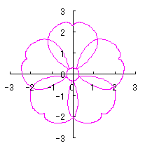
     In order to make overlap among the petals of a flower, it is prefered that the width of a single petal, in another words, the bottom angle of a heart curve to form a petal (which is described in eq.(4)) is intended to be magnified.
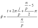
    Therefor, as the magnification factor , the following equation is used instead of Eq.(5).
      .                      (A1)

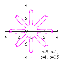
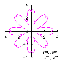
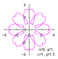
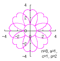
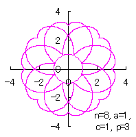
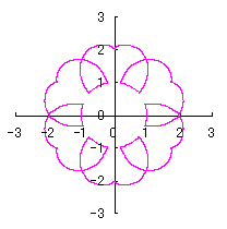
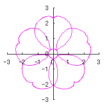
    Then, the (x, y) coordinate data of the shape of a flower are calculated by Eqs.(1), (2), (4), (6), (7) and Eq.(A1),    Examples of such calculated shape of flower in the case of are shown below.

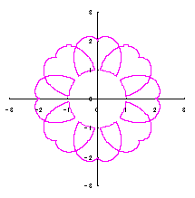
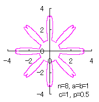
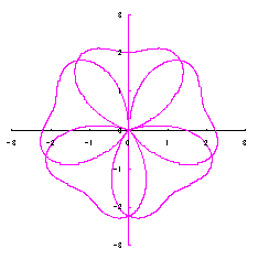
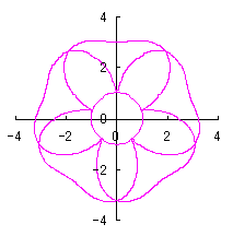
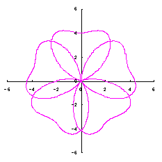
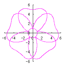
Fig.A1  n=8, a=1, c=1, p=0.5
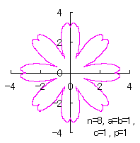
Fig.A2  n=8, a=1, c=1, p=1
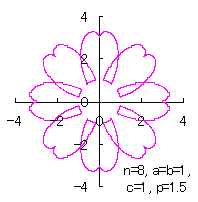
Fig.A3  n=8, a=1, c=1, p=1.5
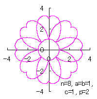
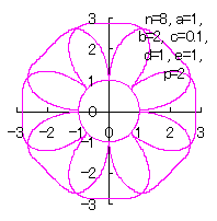
Fig.A4  n=8, a=1, c=1, p=2
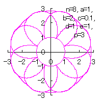
Fig.A5  n=8, a=1, c=1, p=3

     When the above figures are painted, the following ones are drawn.

Fig.A1Fig.A2Fig.A3Fig.A4Fig.A5


     In purpose to calculate the numerical coordinates data of a flower by Eqs.(1), (2), (4), (5), (6) and Eq.(A1), a C++ program is given by C++ program_a_overlap.
    By executing the C++ program, a text file named "flower_a_overlap.txt" including the calculated data is produced.    Each interval of these data is divided by 'comma'.    After moving these calculated data into an excel file, we obtain a heart curve with the use of a graph wizard attached on the excel file.

Added in Sep 21, 2012.


[2.1 Additional II]    In the case that each petal contacts with the center circle with an arbitral width of phase angle of its circle

     The base of petals may actually be connected to the flower floor with a narrow width.    In the simulation of this page, this fact is corresponding to that the petals are connected to a center circle with a narrow width.
    Then, we consider that the petals are in contact to the center circle with an arbitrary phase angle including null phase angle of point contact.    For this purpose, it is prefered that the phase angle of the center circle is independently set to that of the each petal.

    In the case that each petal contacts with the center circle at one point, as the phase angle of the center circle takes the fixed value at the contact point with each petal, then, the following two equations are used instead of Eqs.(6) and (7).    Herein, the reason why the term of exists in this equation is because the central phase of the first () petal is situated at of the phase of the center circle, and then, the count of the phase of the each petal starts from this phase .    In addition, there may be a need to draw a separate center circle connecting each point of each petal in contact with the center circle.
          ,                      (A2)
          ,                      (A3)
where is the radius of the center circle.

    To extend the above, we treat the case that each petal contacts with the center circle with an arbitral angle of its center circle as the following.
    If we take as an arbitral width of phase angle with which each petal contacts to the center circle, the phase angle of the center circle is discribed as , and then, it depends on .
    Accordingly, the following two equations are used instead of Eqs.(A2) and (A3).    In addition, there may be a need to draw a separate center circle connecting each neighbouring petals in the contact region.
          ,                      (A4)
          ,                      (A5)
where is the radius of the center circle and is the fundamental angle with which a single petal occupies the center circle as the angle of round is divided by the number of petals.
    By the way, in calculating C program, we take the correction factor as an input variable, and then, we give the arbitral width of phase angle with which each petal contacts to the center circle.

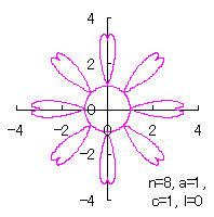
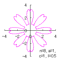
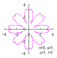
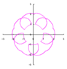
    The (x, y) coordinate data of the shape of a flower are calculated by Eqs.(1), (2), (4), (5), Eqs.(A4) and (A5),    Examples of such calculated shape of flower in the case of are shown below.

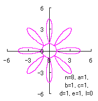
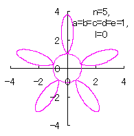
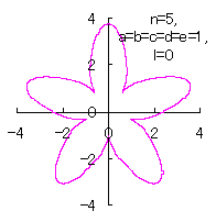
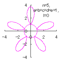
Fig.A6  n=8, a=1, c=1, l=0
Fig.A7  n=8, a=1, c=1, l=0.5
Fig.A8  n=8, a=1, c=1, l=1
Fig.A9  n=8, a=1, c=1, l=2

     In purpose to calculate the numerical coordinates data of a flower by Eqs.(1), (2), (4), (5), (A4) and Eq.(A5), a C++ program is given by C++ program_a_independent_angle.
    By executing the C++ program, a text file named "flower_a_independent_angle.txt" including the calculated data is produced.    Each interval of these data is divided by 'comma'.    After moving these calculated data into an excel file, we obtain a heart curve with the use of a graph wizard attached on the excel file.

Added in Sep. 30, 2012.


2.2    In the case of change in the length and width of heart curve to be used as a petal of flower

     In this case, we return to a heart curve (as shown in Fig.1 and which is used as the material of a petal) in the (x, y) coordinate expression.    This expression is described in the following two equations with the ratio of expansion and contraction in the y direction.
          ,                      (8)
                                (9)
where the phase angle is given by Eq.(3).    In the next, we express the heart curve in the polar coordinates again.    In this case, the moving radius and the phase angle are given by the followings;
          ,                      (10)
          ,                      (11)

     We will arrange such the obtained heart curves as petals of a flower around a center circle of radius .    In the same manner as obtaining Eq.(5), the number is assigned to the each of petals.    Then, the phase angle of -th number's of petal is expressed in the following equation into which the angle described in Eq.(11) is added to .

          .                      (12)

    In the same as Eqs.(6) and (7), a whole flower is expressed in the following two equations in the orthogonal (x, y) coordinates.
          .                      (13)
          .                      (14)

    By the way, as a gap yields between the neighbored two petals when the ratio of expansion and contraction in the y direction mentioned above is not a unit, it may be prefer that the neighbored two petals are connected by an arc of radius .

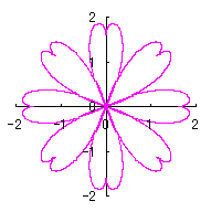
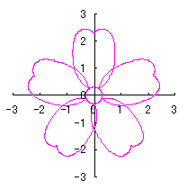
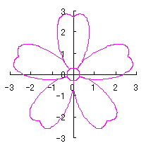
    Then, the (x, y) coordinate data of the shape of a flower are calculated by Eqs.(1) to (3) and Eqs.(8) to (14),    Examples of such calculated shape of flower in the case of are shown below.

Fig.18  n=1, b=0.8, c=0
Fig.19  n=2, b=0.8, c=0
Fig.20  n=3, b=0.8, c=0
Fig.21  n=4, b=0.8, c=0

Fig.22  n=5, b=0.8, c=0
Fig.23  n=5, b=0.5, c=0
Fig.24  n=5, b=0.5, c=1
Fig.25  n=5, b=0.5, c=2

Fig.26a  n=5, b=1, c=2
Fig.26b  n=5, b=1.2, c=2
Fig.27a  n=6, b=0.8, c=0
Fig.27b  n=6, b=0.5, c=0

Fig.27c  n=6, b=0.5, c=1
Fig.28  n=8, b=0.8, c=0
Fig.29  n=8, b=0.5, c=0
Fig.30  n=8, b=0.5, c=1

     When the above figures are painted, the following ones are drawn.      If clicked, an expanded line drawing appears.

Fig.18 n=1, b=0.8, c=0Fig.19 n=2, b=0.8, c=0Fig.20 n=3, b=0.8, c=0Fig.21 n=4, b=0.8, c=0Fig.22 n=5, b=0.8, c=0Fig.23 n=5, b=0.5, c=0Fig.24 n=5, b=0.5, c=1Fig.25 n=5, b=0.5, c=2Fig.26a n=5, b=1, c=2Fig.26b n=5, b=1.2, c=2Fig.27a n=6, b=0.8, c=0Fig.27b n=6, b=0.5, c=0Fig.27c n=6, b=0.5, c=1Fig.28 n=8, b=0.8, c=0Fig.29 n=8, b=0.5, c=0Fig.30 n=8, b=0.5, c=1


     In purpose to calculate the numerical coordinates data of a flower by Eqs.(1) to (3) and Eqs.(8) to (14), a C++ program is given by C++ program_b.
    By executing the C++ program, a text file named "flower_b.txt" including the calculated data is produced.    Each interval of these data is divided by 'comma'.    After moving these calculated data into an excel file, we obtain a heart curve with the use of a graph wizard attached on the excel file.


[2.2 Additional I]

    In the case of overlap among the petals of a flower

     In order to make overlap among the petals of a flower, it is prefered that the width of a single petal, in another words, the angle (which is given by eq.(11)) is intended to be magnified.
     Therefor, as the magnification factor , the following equation is used instead of Eq.(12).
          .                       (B1)

    Then, the (x, y) coordinate data of the shape of a flower are calculated by Eqs.(8) to (11), Eqs.(11), (13), (14) and Eq.(B1),    Examples of such calculated shape of flower in the case of are shown below.

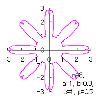
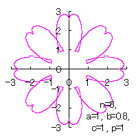
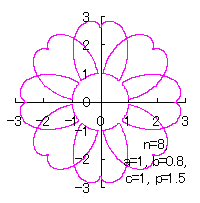
Fig.B1  n=8, a=1, b=0.8, c=1, p=0.5
Fig.B2  n=8, a=1, b=0.8, c=1, p=1
Fig.B3  n=8, a=1, b=0.8, c=1, p=1.5
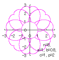
Fig.B4  n=8, a=1, b=0.8, c=1, p=2

Fig.B5  n=8, a=1, b=1, c=1, p=0.5
Fig.B6  n=8, a=1, b=1, c=1, p=1
Fig.B7  n=8, a=1, b=1, c=1, p=1.5
Fig.B8  n=8, a=1, b=1, c=1, p=2

     When the first half part of the above figures is painted, the following figures are drawn.

Fig.B1Fig.B2Fig.B3Fig.B4


     In purpose to calculate the numerical coordinates data of a flower by Eqs.(8) to (11), Eqs.(11), (13), (14) and Eq.(B1), a C++ program is given by C++ program_b_overlap.
    By executing the C++ program, a text file named "flower_b_overlap.txt" including the calculated data is produced.    Each interval of these data is divided by 'comma'.    After moving these calculated data into an excel file, we obtain a heart curve with the use of a graph wizard attached on the excel file.

Added in Sep 21, 2012.
[2.2 Additional II]

     In the case that each petal contacts with the center circle with an arbitral width of phase angle of its circle

    We can describe the solution of this problem as the followings likely as in [2.1 Additional II] of the foregoing section.

     In the case that each petal contacts with the center circle at one point, as the phase angle of the center circle takes the fixed value at the contact point with each petal, then, the following two equations are used instead of Eqs.(13) and (14).    Herein, the reason why the term of exists in this equation is because the central phase of the first () petal is situated at of the phase of the center circle, and then, the count of the phase of the each petal starts from this phase .    In addition, there may be a need to draw a separate center circle connecting each point of each petal in contact with the center circle.
          ,                      (B2)
          ,                      (B3)
where is the radius of the center circle.

    To extend the above, we treat the case that each petal contacts with the center circle with an arbitral angle of its center circle as the following.
    If we take as an arbitral width of phase angle with which each petal contacts to the center circle, the phase angle of the center circle is discribed as , and then, it depends on .
    Accordingly, the following two equations are used instead of Eqs.(B2) and (B3).    In addition, there may be a need to draw a separate center circle connecting each neighbouring petals in the contact region.
          ,                      (B4)
          ,                      (B5)
where is the radius of the center circle and is the fundamental angle with which a single petal occupies the center circle as the angle of round is divided by the number of petals.
    By the way, in calculating C program, we take the correction factor as an input variable, and then, we give the arbitral width of phase angle with which each petal contacts to the center circle.

    The (x, y) coordinate data of the shape of a flower are calculated by Eqs.(1) to (3), Eqs.(8) to (12), Eqs.(B4) and (B5),    Examples of such calculated shape of flower in the case of are shown below.

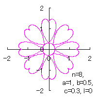
Fig.B9  n=8, a=1, b=0.5,
c=0.3, l=0
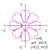
Fig.B10  n=8, a=1, b=0.5,
c=0.3, l=0.5
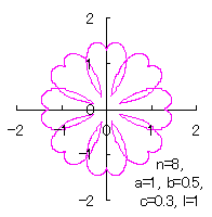
Fig.B11  n=8, a=1, b=0.5,
c=0.3, l=1
Fig.B12  n=8, a=1, b=0.5,
c=0.3, l=2

     In purpose to calculate the numerical coordinates data of a flower by Eqs.(1) to (3), Eqs.(8) to (12), Eqs.(B4) and (B5), a C++ program is given by C++ program_b_independent_angle.
    By executing the C++ program, a text file named "flower_b_independent_angle.txt" including the calculated data is produced.    Each interval of these data is divided by 'comma'.    After moving these calculated data into an excel file, we obtain a heart curve with the use of a graph wizard attached on the excel file.

Added in Oct. 01, 2012.

3.    Method 2

     Method 2 is to make a heart curve from a Cardioid by forming an angle on its bottom in application of some conversion equation of the phase angle, where the heart curve will be used as a petal of a flower,

3.1    In the case of using heart curves as petals of a flower without simplification

    The original Cardioid and the heart curve, which is produced from the original Cardioid by the method 2 as described in the page of "heart curves II", are shown in Fig,31a and Fig.31b respectively.    We intend to form a shape of flower by arranging the heart curves around a center circle.

Fig.31a  The original Cardioid
Fig.31b  Heart curve
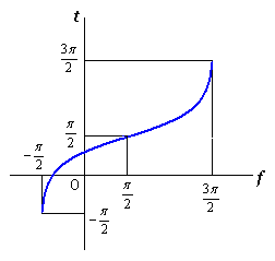
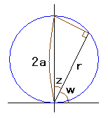
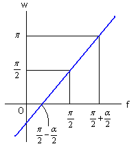
Fig.31c  Conversion of the phase angle
from into

     The equations obtained in the page "heart curves II" and used also in this page are the following three ones;
          ,                      (15)

where .

          .                      (16)
          ,                      (17)
where indicates the phase angle of the heart curve which conversed by Eq.(15) as shown in Fig.31b, the ratio of expansion and contraction in the y direction in regard to the original Cardioid, the coefficient expressing another conversion strength to display the more beautiful heart curve, the ratio of expansion and contraction in the y direction in regard to the conversed heart curve, the moving radius of the original Cardioid expressed in the following equation, and indicates the phase angle of the original Cardioid.
          .                      (18)


Fig.32  Relation between the phase angle of the whole shape of flower
and the phase angle of the heart curve after the displacement of the origin point

    The origin point in Fig.31b is needed to be moved to the bottom of the heart curve.    Although Eq.(16) is not varied in such a displacement, Eq.(17) should be varied in the following equation.
          .                      (19)
    After the displacement of the origin point, the moving radius and the phase angle , which is described as "ff" in the C program below, are written in the following equations;
          .                      (20)
          .                      (21)

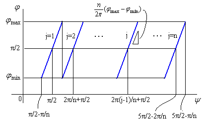
    Next, as we intend that numbers of such the obtained heart curves are arranged around a center circle of radius as petals of a flower, we converse the phase angle of the heart curve, whose origin point has been displaced, into the phase angle of a whole shape of a flower ,which angle is described as "fff" in the C program below.    Such a conversion is illustrated in Fig.32, and is given by
          ,                      (22)
where indicates the -th number's petal of a flower.


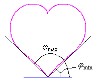
Fig.34  Definition 2 of and
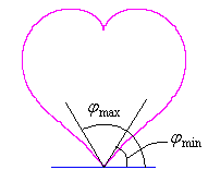
Fig.33  Definition 1 of and

     Newly, the expression of the whole shape of a flower in the orthogonal coordinates are given as
          .                      (23)
          ,                      (24)
where indicates the radius of a center circle surrounded by petals.

    In this time, we treat two cases of using Figs.33 or 34 in regard to the selection of both and , and will separate and discuss in the each case.


3.1.1    In the case using Fig.33

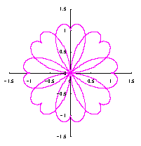
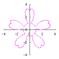
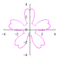
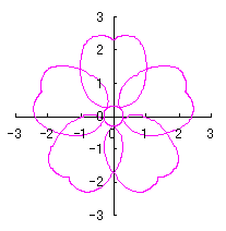
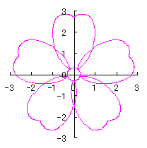
     As seen in Fig.33, the minimum and maximum phase angles of the heart curve possess the proper meanings.    The values of these angles will be obtained by software of C program.    On this base, the (x, y) coordinate data of shape of flower are calculated by Eqs.(15) to (24).    Examples of such calculated shape of flower in the case of are shown below.

Fig.35 n=1, b=1.2, c=0.5, d=1, e=0
Fig.36 n=2, b=1.5, c=0.5, d=1, e=0
Fig.37 n=3, b=1.2, c=0.5, d=1, e=0
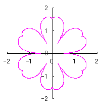
Fig.38 n=4, b=1.4, c=0.5, d=1, e=0

Fig.39 n=5, b=1.5, c=0.3, d=1, e=0
Fig.40 n=5, b=1.5, c=0.3, d=1, e=1
Fig.41 n=5, b=2, c=0.5, d=1, e=0
Fig.42 n=5, b=2, c=0.5, d=1, e=0.5

Fig.43 n=5, b=2.2, c=0.7, d=1, e=0
Fig.44 n=5, b=2.2, c=0.7, d=1, e=1
Fig.45a n=5, b=3, c=0.9, d=1, e=0
Fig.45b n=5, b=3, c=0.9, d=1, e=0.5

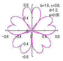
Fig.46 n=5, b=1.8, c=0.8, d=1.2,
e=0.05
Fig.47a n=6, b=2, c=0.5, d=1, e=0
Fig.47b n=6, b=2, c=0.5, d=1, e=0.5
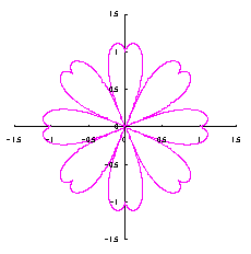
Fig.48a n=8, b=2, c=0.5, d=1, e=0
Fig.48b n=8, b=2, c=0.5, d=1, e=0.5

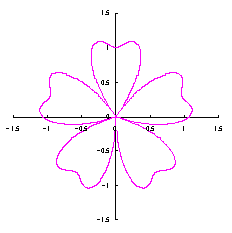
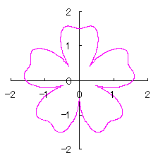
     When the above figures are painted, the following ones are drawn.    If clicked, an expanded line drawing appears.

wood sorrel
Fig.35 n=1, b=1.2, c=0.5, d=1, e=0Fig.36 n=2, b=1.5, c=0.5, d=1, e=0Fig.37 n=3, b=1.2, c=0.5, d=1, e=0Fig.38 n=4, b=1.4, c=0.5, d=1, e=0Fig.39 n=5, b=1.5, c=0.3, d=1, e=0Fig.39 n=5, b=1.5, c=0.3, d=1, e=0Fig.41 n=5, b=2, c=0.5, d=1, e=0Fig.42 n=5, b=2, c=0.5, d=1, e=0.5Fig.43 n=5, b=2.2, c=0.7, d=1, e=0Fig.44 n=5, b=2.2, c=0.7, d=1, e=1Fig.45a n=5, b=3, c=0.9, d=1, e=0Fig.45b n=5, b=3, c=0.9, d=1, e=0.5Fig.46Fig.47a n=6, b=2, c=0.5, d=1, e=0Fig.47b n=6, b=2, c=0.5, d=1, e=0.5Fig.48a n=8, b=2, c=0.5, d=1, e=0Fig.48b n=8, b=2, c=0.5, d=1, e=0.5

     In purpose to calculate the numerical coordinates data of a flower by Eqs.(15) to (24), a C++ program is given by C++ program_c1.
    By executing the C++ program, a text file named "flower_c1.txt" including the calculated data is produced.    Each interval of these data is divided by 'comma'.    After moving these calculated data into an excel file, we obtain a heart curve with the use of a graph wizard attached on the excel file.


[3.1.1 Additional I]   In the case of overlap among the petals of a flower

    In order to make overlap among the petals of a flower, it is prefered that the width of a single petal is intended to be increased.    If the inclination of the lines in Fig.32 is increased, the width of a single petal is increased.
    Therefor, as the inclimentation factor of this inclination, the following equation is used instead of Eq.(22).
          .                      (C1)

    Then, the (x, y) coordinate data of the shape of a flower are calculated by Eqs.(15) to (21), Eqs.(23), (24) and Eq.(C1),    Examples of such calculated shape of flower in the case of are shown below.

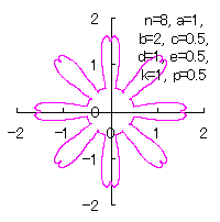
Fig.CI1  n=8, a=1, b=2, c=0.5,
d=1, e=0.5, k=1, p=0.5
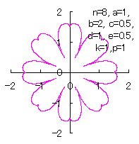
Fig.CI2  n=8, a=1, b=2, c=0.5,
d=1, e=0.5, k=1, p=1
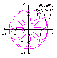
Fig.CI3  n=8, a=1, b=2, c=0.5,
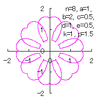
d=1, e=0.5, k=1, p=1.5
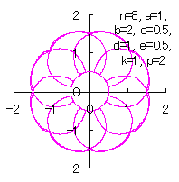
Fig.CI4  n=8, a=1, b=2, c=0.5,
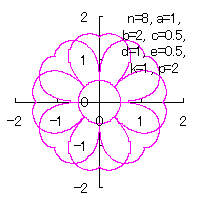
d=1, e=0.5, k=1, p=2

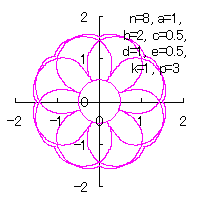
Fig.CI5  n=8, a=1, b=2, c=0.5,
d=1, e=0.5, k=1, p=3
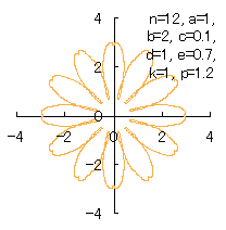
Fig.CI6  n=12, a=1, b=2, c=0.1,
d=1, e=0.7, k=1, p=1.2

     When the above figures are painted, the following ones are drawn.

Fig.CI1Fig.CI2Fig.CI3Fig.CI4Fig.CI5Fig.CI6reference to Fig.CI6

     In purpose to calculate the numerical coordinates data of a flower by Eqs.(15) to (21), Eqs.(23), (24) and Eq.(C1), a C++ program is given by C++ program_c1_overlap.
    By executing the C++ program, a text file named "flower_c1_overlap.txt" including the calculated data is produced.    Each interval of these data is divided by 'comma'.    After moving these calculated data into an excel file, we obtain a heart curve with the use of a graph wizard attached on the excel file.

Added in Sep 22, 2012.

[3.1.1 Additional II]    In the case that each petal contacts with the center circle with an arbitral width of phase angle of its circle

     We can describe the solution of this problem as the followings likely as in [2.1 Additional II] of the section 2.1 and likely as in [2.2 Additional II] of the foregoing section.

    In the case that each petal contacts with the center circle at one point, as the phase angle of the center circle takes the fixed value at the contact point with each petal, then, the following two equations are used instead of Eqs.(23) and (24).    Herein, the reason why the term of exists in this equation is because the central phase of the first () petal is situated at of the phase of the center circle, and then, the count of the phase of the each petal starts from this phase .    In addition, there may be a need to draw a separate center circle connecting each point of each petal in contact with the center circle.
          ,                      (CI2)
          ,                      (CI3)
where is the radius of the center circle.

    To extend the above, we treat the case that each petal contacts with the center circle with an arbitral angle of its center circle as the following.
    If we take as an arbitral width of phase angle with which each petal contacts to the center circle, the phase angle of the center circle is discribed as , and then, it depends on .
    Accordingly, the following two equations are used instead of Eqs.(CI2) and (CI3).    In addition, there may be a need to draw a separate center circle connecting each neighbouring petals in the contact region.
          ,                      (CI4)
          ,                      (CI5)
where is the radius of the center circle and is the fundamental angle with which a single petal occupies the center circle as the angle of round is divided by the number of petals.
    By the way, in calculating C program, we take the correction factor as an input variable, and then, we give the arbitral width of phase angle with which each petal contacts to the center circle.

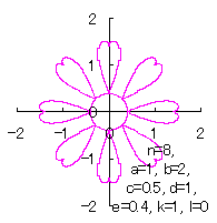
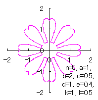
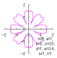
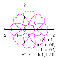
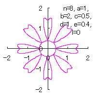
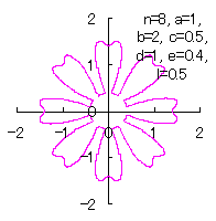
    The (x, y) coordinate data of the shape of a flower are calculated by Eqs.(15) to (22), Eqs.(CI4) and (CI5),    Examples of such calculated shape of flower in the case of are shown below.

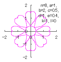
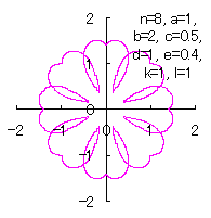
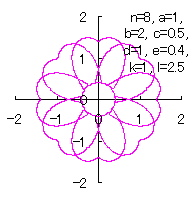
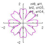
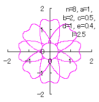
Fig.CI7  n=8, a=1, b=2, c=0.5,
d=1, e=0.4, k=1, l=0
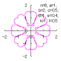
Fig.CI8  n=8, a=1, b=2, c=0.5,
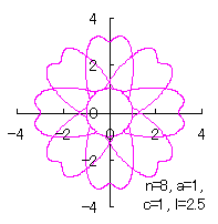
d=1, e=0.4, k=1, l=0.5
Fig.CI9  n=8, a=1, b=2, c=0.5,
d=1, e=0.4, k=1, l=1
Fig.CI10  n=8, a=1, b=2, c=0.5,
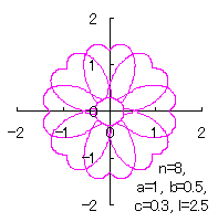
d=1, e=0.4, k=1, l=2.5

     In purpose to calculate the numerical coordinates data of a flower by Eqs.(15) to (22), Eqs.(C14) and (C15), a C++ program is given by C++ program_c1_independent_angle.
    By executing the C++ program, a text file named "flower_c1_independent_angle.txt" including the calculated data is produced.    Each interval of these data is divided by 'comma'.    After moving these calculated data into an excel file, we obtain a heart curve with the use of a graph wizard attached on the excel file.

Added in Oct. 01, 2012.

3.1.2    In the case using Fig.34

     As seen in Fig.34, as the minimum and maximum phase angles are defined at the bottom of the heart curve, the values of these angles are generally different from ones described in the section 3.1.1.    These angles are obtained analytically as
          ,                      (25)
and
          .                      (26)
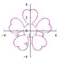
    The (x, y) coordinate data of shapes of flower are calculated by Eqs.(15) to (26),    Examples of such calculated shape of flower in the case of are shown below.

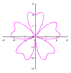
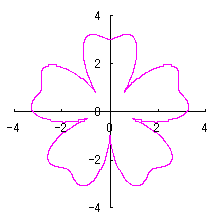
Fig.49 n=1, b=1, c=0.5, d=1, e=0
Fig.50 n=2, b=1, c=0.5, d=1, e=0
Fig.51 n=3, b=1, c=0.5, d=1, e=0
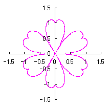
Fig.52 n=4, b=1, c=0.5, d=1, e=0

Fig.53 n=5, b=1, c=0.5, d=1, e=0.5
Fig.54 n=5, b=1, c=0.5, d=1, e=1
Fig.55 n=5, b=2, c=0.5, d=0.5, e=0
Fig.56 n=5, b=2, c=0.5, d=0.5, e=1

Fig.57 n=5, b=2, c=0.5, d=1, e=0
Fig.58 n=5, b=2, c=0.5, d=1, e=1.5
Fig.59a n=6, b=1, c=0.5, d=1, e=0
Fig.59b n=6, b=2, c=0.5, d=1, e=0

Fig.59c n=6, b=2, c=0.5, d=1, e=0.5
Fig.60a n=8, b=1, c=0.5, d=1, e=0
Fig.60b n=8, b=2, c=0.5, d=1, e=0
Fig.60c n=8, b=2, c=0.5, d=1, e=0.5

    When the above figures are painted, the following ones are drawn.    If clicked, an expanded line drawing appears.

young leaves of clover
Fig.49 n=1, b=1, c=0.5, d=1, e=0Fig.50 n=2, b=1, c=0.5, d=1, e=0Fig.51 n=3, b=1, c=0.5, d=1, e=0Fig.52 n=4, b=1, c=0.5, d=1, e=0Fig.53 n=5, b=1, c=0.5, d=1, e=0Fig.54 n=5, b=1, c=0.5, d=1, e=1Fig.55 n=5, b=2, c=0.5, d=0.5, e=0Fig.56 n=5, b=2, c=0.5, d=0.5, e=1Fig.57 n=5, b=2, c=0.5, d=1, e=0Fig.58 n=5, b=2, c=0.5, d=1, e=1.5Fig.59a n=6, b=1, c=0.5, d=1, e=0Fig.59b n=6, b=2, c=0.5, d=1, e=0Fig.59c n=6, b=2, c=0.5, d=1, e=0.5Fig.60a n=8, b=1, c=0.5, d=1, e=0Fig.60b n=8, b=2, c=0.5, d=1, e=0Fig.60c n=8, b=2, c=0.5, d=1, e=0.5


     In purpose to calculate the numerical coordinates data of a flower by Eqs.(15) to (26), a C++ program is given by C++ program_c2.
    By executing the C++ program, a text file named "flower_c2.txt" including the calculated data is produced.    Each interval of these data is divided by 'comma'.    After moving these calculated data into an excel file, we obtain a heart curve with the use of a graph wizard attached on the excel file.


[3.1.2 Additional I]   In the case of overlap among the petals of a flower

     We can use all the equations of Eqs.(15) to (21), Eqs.(23), (24) and Eq.(C1) as likely as used in the 3.1.1 Additional,
    Moreover, we use Eqs.(25) and (26) described just above.

    Then, the (x, y) coordinate data of the shape of a flower are calculated by from Eqs.(15) to (21), Eqs.(23) and (24), Eq.(C1), Eqs.(25) and (26),    Examples of such calculated shape of flower in the case of are shown below.

Fig.CII1  n=8, a=1, b=2, c=0.5,
d=1, e=0.5, k=1, p=0.5
Fig.CII2  n=8, a=1, b=2, c=0.5,
d=1, e=0.5, k=1, p=1
Fig.CII3  n=8, a=1, b=2, c=0.5,
d=1, e=0.5, k=1, p=1.5
Fig.CII4  n=8, a=1, b=2, c=0.5,
d=1, e=0.5, k=1, p=2

     When the above figures are painted, the following ones are drawn.

図CII1図CII2図CII3図CII4

     In purpose to calculate the numerical coordinates data of a flower by Eqs.(15) to (21), Eqs.(23) and (24), Eq.(C1), Eqs.(25) and (26), a C++ program is given by C++ program_c2_overlap.
    By executing the C++ program, a text file named "flower_c2_overlap.txt" including the calculated data is produced.    Each interval of these data is divided by 'comma'.    After moving these calculated data into an excel file, we obtain a heart curve with the use of a graph wizard attached on the excel file.

Added in Sep 22, 2012.

[3.1.2 Additional II]    In the case that each petal contacts with the center circle with an arbitral width of phase angle of its circle

     We can describe the solution of this problem as the followings likely as in [2.1 Additional II] of the section 2.1, likely as in [2.2 Additional II] of the the section 2.2 and likely as in [3.1.1 Additional II] of the foregoing section.

    In the case that each petal contacts with the center circle at one point, as the phase angle of the center circle takes the fixed value at the contact point with each petal, then, the following two equations are used instead of Eqs.(23) and (24).    Herein, the reason why the term of exists in this equation is because the central phase of the first () petal is situated at of the phase of the center circle, and then, the count of the phase of the each petal starts from this phase .    In addition, there may be a need to draw a separate center circle connecting each point of each petal in contact with the center circle.
          ,                      (CII1)
          ,                      (CII2)
where is the radius of the center circle.

    To extend the above, we treat the case that each petal contacts with the center circle with an arbitral angle of its center circle as the following.
    If we take as an arbitral width of phase angle with which each petal contacts to the center circle, the phase angle of the center circle is discribed as , and then, it depends on .
    Accordingly, the following two equations are used instead of Eqs.(CII1) and (CII2).    In addition, there may be a need to draw a separate center circle connecting each neighbouring petals in the contact region.
          ,                      (CII3)
          ,                      (CII4)
where is the radius of the center circle and is the fundamental angle with which a single petal occupies the center circle as the angle of round is divided by the number of petals.
    By the way, in calculating C program, we take the correction factor as an input variable, and then, we give the arbitral width of phase angle with which each petal contacts to the center circle.

    The (x, y) coordinate data of the shape of a flower are calculated by Eqs.(15) to (22), Eq.(25), Eq.(26), Eqs.(CII3) and (CII4),    Examples of such calculated shape of flower in the case of are shown below.

Fig.CII5  n=8, a=1, b=2, c=0.5,
d=1, e=0.4, k=1, l=0
Fig.CII6  n=8, a=1, b=2, c=0.5,
d=1, e=0.4, k=1, l=0.5
Fig.CII7  n=8, a=1, b=2, c=0.5,
d=1, e=0.4, k=1, l=1
Fig.CII8  n=8, a=1, b=2, c=0.5,
d=1, e=0.4, k=1, l=2.5

     In purpose to calculate the numerical coordinates data of a flower by Eqs.(15) to (22), Eq.(25), Eq.(26), Eqs.(CII3) and (CII4), a C++ program is given by C++ program_c2_independent_angle.
    By executing the C++ program, a text file named "flower_c2_independent_angle.txt" including the calculated data is produced.    Each interval of these data is divided by 'comma'.    After moving these calculated data into an excel file, we obtain a heart curve with the use of a graph wizard attached on the excel file.

Added in Oct. 01, 2012.

3.2    In the case of using heart curves as petals of a flower with simplification

     The process treating in the previous section 3.1 is a little complicated for holding a correct shape of heart curve.    So, we divert the phase angle , which is given by Eq.(12) as an angle before conversion, instead of the correct phase angle , which is given by Eq.(22) and is shown in Fig.32, as a phase angle of shape of a flower.    The conversion of the phase angle from (a single heart curve expressed in Fig.31b) into (the shape of a flower) is like that , and are replaced to , and respectively in Eq.(22).
          ,                      (27)
where indicates the -th number's petal of a flower.
    On th other hand, the moving radius is obeyed to the precise process given by Eq.(20).
    Then, although the precise description of heart curve is lost, there is some taste in the obtained shape of flower.    As the phase angle is used, the following two equations are replaced to Eqs.(23) and (24).
          .                      (28a)
          .                      (28b)

    Calculating Eqs.(15) to (20), Eqs.(27), (28a) and (28b), examples of shape of flower in the case of are obtained as shown below.

Fig.61 n=5, b=2, c=0.5, d=1, e=0
Fig.61b n=5, b=2, c=0.5, d=1, e=0.5
Fig.62 n=5, b=2, c=0.5, d=1, e=1
Fig.63 n=5, b=2, c=0.7, d=1, e=0

Fig.64 n=5, b=2, c=0.7, d=1, e=0.5
Fig.65 n=8, b=2, c=0.1, d=1, e=0
Fig.66 n=8, b=2, c=0.1, d=1, e=0.5

    When the above figures are painted, the following ones are drawn.    If clicked, an expanded line drawing appears.
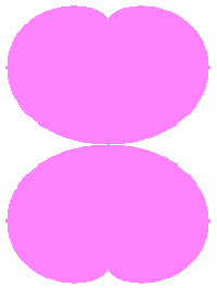

Fig.61 n=5, b=2, c=0.5, d=1, e=0Fig.67b n=5, b=2, c=0.5, d=1, e=0.5Fig.62 n=5, b=2, c=0.5, d=1, e=1 Fig.63 n=5, b=2, c=0.7, d=1, e=0Fig.64 n=5, b=2, c=0.7, d=1, e=0.5Fig.65 n=8, b=2, c=0.1, d=1, e=0Fig.66 n=8, b=2, c=0.1, d=1, e=0.5

     In purpose to calculate the numerical coordinates data of a flower by Eqs.(15) to (20), Eqs.(27), (28a) and (28b), a C++ program is given by C++ program_d.
    By executing the C++ program, a text file named "flower_d.txt" including the calculated data is produced.    Each interval of these data is divided by 'comma'.    After moving these calculated data into an excel file, we obtain a heart curve with the use of a graph wizard attached on the excel file.


[3.2 Additional I]   In the case of overlap among the petals of a flower

    We can also use all the equations of From Eqs.(15) to (21) and Eq.(C1) as likely as used in the 3.1.1 Additional,
    Moreover, we use Eqs.(27) and (28) described just above.

    Then, the (x, y) coordinate data of the shape of a flower are calculated by Eqs.(15) to (21), Eq.(C1), Eqs.(27) and (28),    Examples of such calculated shape of flower in the case of are shown below.

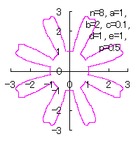
Fig.D1  n=8, a=1, b=2,
c=0.1, d=1, e=1, p=0.5
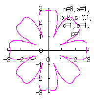
Fig.D2  n=8, a=1, b=2,
c=0.1, d=1, e=1, p=1
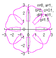
Fig.D3  n=8, a=1, b=2,
c=0.1, d=1, e=1, p=1.5
Fig.D4  n=8, a=1, b=2,
c=0.1, d=1, e=1, p=2
Fig.D4  n=8, a=1, b=2,
c=0.1, d=1, e=1, p=3

    When the above figures are painted, the following ones are drawn.

Fig.D1Fig.D2Fig.D3Fig.D4Fig.D5

     In purpose to calculate the numerical coordinates data of a flower by Eqs.(15) to (21), Eq.(C1), Eqs.(27) and (28), a C++ program is given by C++ program_d_overlapflower_d_overlap.txt" including the calculated data is produced.    Each interval of these data is divided by 'comma'.    After moving these calculated data into an excel file, we obtain a heart curve with the use of a graph wizard attached on the excel file.

Addid in Sep 22, 2012.

[3.2 Additional II]    In the case that each petal contacts with the center circle with an arbitral width of phase angle of its circle

     We can describe the solution of this problem as the followings likely as in [2.1 Additional II] of the section 2.1, likely as in [2.2 Additional II] of the the section 2.2 and likely as in [3.1.1 Additional II] of the foregoing section.

    In the case that each petal contacts with the center circle at one point, as the phase angle of the center circle takes the fixed value at the contact point with each petal, then, the following two equations are used instead of Eqs.(28a) and (28b).    Herein, the reason why the term of exists in this equation is because the central phase of the first () petal is situated at of the phase of the center circle, and then, the count of the phase of the each petal starts from this phase .    In addition, there may be a need to draw a separate center circle connecting each point of each petal in contact with the center circle.
          ,                      (D1)
          ,                      (D2)
where is the radius of the center circle.

    To extend the above, we treat the case that each petal contacts with the center circle with an arbitral angle of its center circle as the following.
    If we take as an arbitral width of phase angle with which each petal contacts to the center circle, the phase angle of the center circle is discribed as , and then, it depends on .
    Accordingly, the following two equations are used instead of Eqs.(D1) and (D2).    In addition, there may be a need to draw a separate center circle connecting each neighbouring petals in the contact region.
          ,                      (D3)
          .                      (D4)
where is the radius of the center circle and is the fundamental angle with which a single petal occupies the center circle as the angle of round is divided by the number of petals.
    By the way, in calculating C program, we take the correction factor as an input variable, and then, we give the arbitral width of phase angle with which each petal contacts to the center circle.

    The (x, y) coordinate data of the shape of a flower are calculated by Eqs.(15) to (21), Eq.(27), Eqs.(D3) and (D4),    Examples of such calculated shape of flower in the case of are shown below.

Fig.D5  n=8, a=1, b=2,
c=0.5, d=1, e=0.4, l=0
Fig.D6  n=8, a=1, b=2,
c=0.5, d=1, e=0.4, l=0.5
Fig.D7  n=8, a=1, b=2,
c=0.5, d=1, e=0.4, l=1
Fig.D8  n=8, a=1, b=2,
c=0.5, d=1, e=0.4, l=2.5


     In purpose to calculate the numerical coordinates data of a flower by Eqs.(15) to (21), Eq.(27), Eqs.(D3) and (D4), a C++ program is given by C++ program_d_independent_angle.
    By executing the C++ program, a text file named "flower_d_independent_angle.txt" including the calculated data is produced.    Each interval of these data is divided by 'comma'.    After moving these calculated data into an excel file, we obtain a heart curve with the use of a graph wizard attached on the excel file.

Added in Oct. 02, 2012.

4.    In the case of using Cardioid directly as a petal of flower

     In this section, we treat the case of using Cardioid directly as a petal of flower.

    After the origin point of Cardioid shown in Fig.1a and given by Eq.(18) is moved to the bottom of the Cardioid, the equations expressing the Cardioid is given by the followings;
          .                      (29)
          ,                      (30)
where is the ratio of expansion and contraction in the y direction likely as in Eq.(17), and the last term in the parenthesis of Eq.(30) is intended to move the origin to the bottom of the Cardioid.

    From the above equations, the moving radius is given by
          .                      (31)
    Then, the equations expressing the shape of a flower are described as the followings instead of Eqs.(23) and (24).
          ,                      (32)
and
          ,                      (33)
where indicates the phase angle around the shape of a flower and indicates the radius of a center circle surrounded by petals.

    In this time, we treat two cases of conversion of the phase angle from (that of a single Cardioid) to (that of the shape of a flower).
    One is the case of no overlap among the petals and another is the case of overlap among the petals.


4.1    In the case of no overlap among the petals of a flower

     The conversion of the phase angle from (that of a single Cardioid) to (that of the shape of a flower) is like that , and are replaced to , t and respectively in Eq.(22).
          ,                      (34)
where indicates the -th number's petal of a flower.    Here, as the movement of the origin point does not give influence to the conversion of the phase angle for simplification, the each petal is not taken over the original Cardioid.

    Calculating Eqs.(29) to (34), examples of shape of flower in the case of are obtained as shown below.

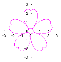
Fig.67 n=5, d=1, e=0
Fig.68 n=5, d=1, e=1
Fig.69 n=5, d=2, e=0
Fig.70 n=5, d=2, e=1

    When the above figures are painted, the following ones are drawn.    If clicked, an expanded line drawing appears.

Fig.67 n=5, d=1, e=0Fig.68 n=5, d=1, e=1Fig.69 n=5, d=2, e=0Fig.70 n=5, d=2, e=1


     In purpose to calculate the numerical coordinates data of a flower by Eqs.(29) to (34), a C++ program is given by C++ program_e1.
    By executing the C++ program, a text file named "flower_e1.txt" including the calculated data is produced.    Each interval of these data is divided by 'comma'.    After moving these calculated data into an excel file, we obtain a heart curve with the use of a graph wizard attached on the excel file.


4.2    In the case of overlap among the petals of a flower

    In this case, the conversion of the phase angle from (that of a Cardioid) to (that of the shape of a flower) is like that and are replaced to and respectively in Eq.(34).
          ,                      (35-1)
where indicates the -th number's petal of a flower.    Likely as in the previous section 4.1, as the movement of the origin point does not make influence to the conversion of the phase angle for simplification, the each petal is not taken over the original Cardioid.

    Further, as an index of the overlap, the evolved equation of Eq.(35-1) is shown in the following.
          ,                      (35-2)
where indicates the -th number's petal of a flower.    Then, for example, the index is specified as in the case of the previous section 4.1 and specified as in the case that adjacent petals are fully overlapped.

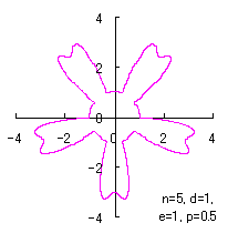
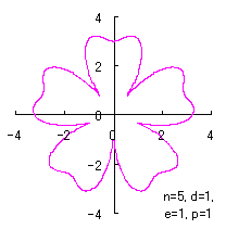
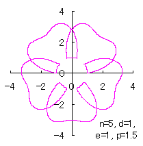
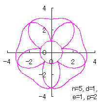
    Calculating Eq.(18), Eqs.(29) to (33) and either Eq.(35-1) or Eq.(35-1), examples of shape of flower in the case of are obtained as shown below.

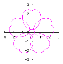
Fig.71a n=5, d=1, e=0
Fig.71b n=5, d=1, e=1
Fig.71c n=5, d=2, e=0
Fig.71d n=5, d=2, e=1

Fig.72 n=6, d=2, e=1  
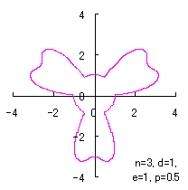
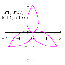
Fig.73a n=3, d=1, e=1, p=0.5  
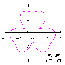
Fig.73b n=3, d=1, e=1, p=1  
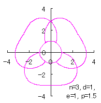
Fig.73c n=3, d=1, e=1, p=1.5  

Fig.74a n=5, d=1, e=1, p=0.5  
Fig.74b n=5, d=1, e=1, p=1  
Fig.74c n=5, d=1, e=1, p=1.5  
Fig.74d n=5, d=1, e=1, p=2  

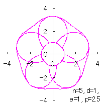
Fig.74e n=5, d=1, e=1, p=2.5  
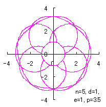
Fig.74f n=5, d=1, e=1, p=3.5  
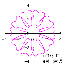
Fig.75a n=10, d=1, e=1, p=1.5  
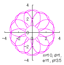
Fig.75b n=10, d=1, e=1, p=3.5  

     When the above figures are painted, the following ones are drawn.     If clicked, a line drawing appears.

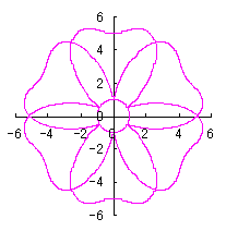
Fig.71a n=5, d=1, e=0Fig.71b n=5, d=1, e=1Fig.71c n=5, d=2, e=0Fig.71d n=5, d=2, e=1Fig.72 n=6, d=2, e=1Fig.73a n=3, d=1, e=1, p=0.5Fig.73b n=3, d=1, e=1, p=1Fig.73c n=3, d=1, e=1, p=1.5Fig.74a n=5, d=1, e=1, p=0.5Fig.74b n=5, d=1, e=1, p=1Fig.74c n=5, d=1, e=1, p=1.5Fig.74d n=5, d=1, e=1, p=2Fig.74e n=5, d=1, e=1, p=2.5Fig.74f n=5, d=1, e=1, p=3.5Fig.75a n=10, d=1, e=1, p=1.5Fig.75b n=10, d=1, e=1, p=3.5


     In purpose to calculate the numerical coordinates data of a flower by Eq.(18), Eqs.(29) to (33) and Eq.(35-2), a C++ program is given by C++ program_e2.
    By executing the C++ program, a text file named "C++ program_e2.txt" including the calculated data is produced.    Each interval of these data is divided by 'comma'.    After moving these calculated data into an excel file, we obtain a heart curve with the use of a graph wizard attached on the excel file.

edited in Mar. 15, 2009 & reviced in Sep. 11, 2012

4.3    In the case that each petal contacts with the center circle with an arbitral width of phase angle of its circle

     We can also use Eq.(18) and Eqs.(29) to (33).
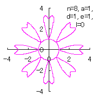
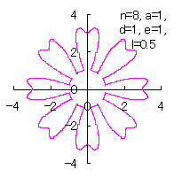
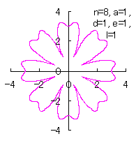
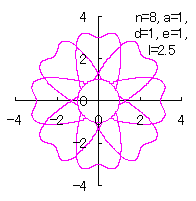
    Moreover, we can consider the solution of this problem as followgs likely as in [3.2 Additional II] of the section 3.2.    So, we also use Eqs.(D3) and (D4).
    In culculating C program, we take the correction factor as an input variable, and then, we give the arbitral width of phase angle with which each petal contacts to the center circle.

    The (x, y) coordinate data of the shape of a flower are calculated by Eq.(18), Eqs.(29) to (33), Eqs.(D3) and (D4),     Examples of such calculated shape of flower in the case of are shown below.

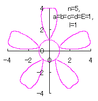
Fig.E1  n=8, a=1, d=1, e=1, l=0
Fig.E2  n=8, a=1, d=1, e=1, l=0.5
Fig.E3  n=8, a=1, d=1, e=1, l=1
Fig.E4  n=8, a=1, d=1, e=1, l=2.5

     In purpose to calculate the numerical coordinates data of a flower by Eq.(18), Eqs.(29) to (33), Eqs.(D3) and (D4), a C++ program is given by C++ program_e_independent_angle.
    By executing the C++ program, a text file named "C++ program_e_independent_angle.txt" including the calculated data is produced.    Each interval of these data is divided by 'comma'.    After moving these calculated data into an excel file, we obtain a heart curve with the use of a graph wizard attached on the excel file.

Added in Oct. 02, 2012.


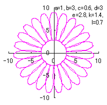
5.     In the case of using a circle directly as a petal of flower


    In this section, we treat the case of using a circle directly as a petal of flower.

    A circle (having the moving radius and the phase angle ) is expressed as .     In the first, we move the origin point from the center to the bottom of a circle.    As a circle itself is too simple to apply to a shape of petal, we introduce the coefficients and as like as Eqs.(16) and (17) and intend to deform a circle by using these coefficients.    Such a deformation is equipped in three kinds and the each kind is treated separately in the respective section below.


5.1    The first deformation of a circle used as a petal

    We assume a deformed circle given by the followings in the orthogonal coordinates;
          .                      (36)
          ,                      (37)
where the last term in the parenthesis of Eq.(37) is intended to move the origin to the bottom of the deformed circle.

    Then, Eq.(31) can be diverted as the moving radius after moving the origin point.     Eqs.(32) and (33) is also diverted as the expression giving a shape of a flower in the orthogonal coordinates where indicates the phase angle around the shape of a flower and e indicates the radius of a center circle surrounded by petals.

    As likely as in the previous section, we treat two cases of conversion of the phase angle from (that of a circle) to (that of the shape of a flower).
    One is the case of no overlap among the petals and another is the case of overlap among the petals.

5.1.1    In the case of no overlap among the petals of a flower

    Eq.(34) can be used as the equation of transformation from (the phase angle of a circle) to (the phase angle around the shape of a flower), where has to be replaced to .

    Calculating Eqs.(31) to (34), Eqs.(36) and (37), examples of shape of flower in the case of are obtained as shown below.

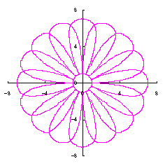
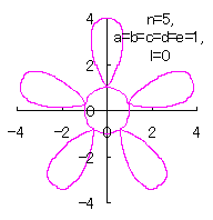
Fig.76 n=5, b=0, c=1, d=2, e=1
Fig.77 n=12, b=0, c=1, d=2, e=1
Fig.78 n=16, b=0, c=4.2, d=3, e=1
Fig.79 n=16, b=0, c=5, d=3, e=1

Fig.80 n=16, b=0.2, c=3.8, d=3, e=1
Fig.81 n=16, b=0.3, c=3, d=3, e=1
Fig.82 n=16, b=0.3, c=4, d=3, e=1

     When the above figures are painted, the following ones are drawn.    If clicked, an expanded line drawing appears.

Fig.76 n=5, b=0, c=1, d=2, e=1Fig.77 n=12, b=0, c=1, d=2, e=1Fig.78 n=16, b=0, c=4.2, d=3, e=1Fig.79 n=16, b=0, c=5, d=3, e=1Fig.80 n=16, b=0.2, c=3.8, d=3, e=1Fig.81 n=16, b=0.3, c=3, d=3, e=1Fig.82 n=16, b=0.3, c=4, d=3, e=1


     In purpose to calculate the numerical coordinates data of a flower by Eqs.(31) to (34), Eqs.(36) and (37), a C++ program is given by C++ program_f1.
    By executing the C++ program, a text file named "C++ program_f1.txt" including the calculated data is produced.    Each interval of these data is divided by 'comma'.    After moving these calculated data into an excel file, we obtain a heart curve with the use of a graph wizard attached on the excel file.


5.1.2    In the case of overlap among the petals of a flower

     In this case, Eq.(35-1) or (35-2) can be used as the equation of transformation from (the phase angle of a circle) to (the phase angle around the shape of a flower), where has to be replaced to .

    Calculating Eqs.(31) to (33), either Eq.(35-1) or Eq.(35-2), Eqs.(36) and (37), examples of shape of flower in the case of are obtained as shown below.

Fig.83 n=5, b=0, c=1,
d=2, e=0, p=2
Fig.84 n=5, b=0, c=1,
d=2, e=1, p=2
Fig.85a n=16, b=0.2, c=3.8,
d=3, e=1, p=2
Fig.85b n=32, b=0.2, c=3.8,
d=3, e=1, p=2

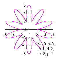
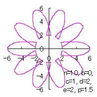
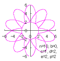
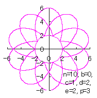
Fig.86a n=10, b=0, c=1,
d=2, e=2,
p=0.5
Fig.86b n=10, b=0, c=1,
d=2, e=2,
p=1
Fig.86c n=16, b=0, c=1,
d=2, e=2,
p=1.5
Fig.86d n=10, b=0, c=1,
d=2, e=2,
p=2

Fig.86e n=10, b=0, c=1,
d=2, e=2,
p=3
Fig.86f n=10, b=0, c=1,
d=2, e=2,
p=4

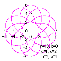
     When the above figures of Figs.85 to 83b and Fig.96f are painted, they are drawn as in the folloings.    If the each of four figures in the left side is clicked, an expanded line drawing appears.

Fig.83 n=5, b=0, c=1, d=2, e=0Fig.84 n=5, b=0, c=1, d=2, e=1Fig.85a n=16, b=0.2, c=3.8, d=3, e=1Fig.85b n=32, b=0.2, c=3.8, d=3, e=1Fig.86f n=10, b=0, c=1, d=2, e=2, p=4


     In purpose to calculate the numerical coordinates data of a flower by from Eqs.(31) to (33), Eqs.(35-2), (36) and (37), a C++ program is given by C++ program_f2.
     By executing the C++ program, a text file named "C++ program_f2.txt" including the calculated data is produced.    Each interval of these data is divided by 'comma'.    After moving these calculated data into an excel file, we obtain a heart curve with the use of a graph wizard attached on the excel file.

edited in Mar. 15, 2009 & reviced in Sep. 14, 2012


5.1.3    In the case that each petal contacts with the center circle with an arbitral width of phase angle of its circle

     We can also use Eqs.(27), (31), (36) and (37).
    Moreover, we can consider the solution of this problem as followgs likely as in [3.2 Additional II] of the section 3.2.    So, we also use Eqs.(D3) and (D4).
    In calculating C program, we take the correction factor as an input variable, and then, we give the arbitral width of phase angle with which each petal contacts to the center circle.

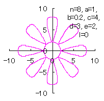
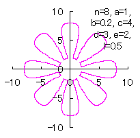
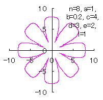
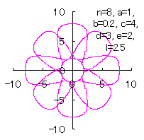
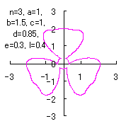
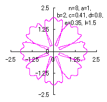
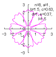
    The (x, y) coordinate data of the shape of a flower are calculated by Eqs.(27), (31), (36), (37), Eqs.(D3) and (D4),     Examples of such calculated shape of flower in the case of are shown below.

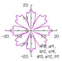
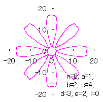
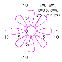
Fig.F1a  n=8, a=1, b=0.2, c=4,
d=3, e=2, l=0
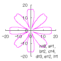
Fig.F1b  n=8, a=1, b=0.2, c=4,
d=3, e=2, l=0.5
Fig.F1c  n=8, a=1, b=0.2, c=4,
d=3, e=2, l=1
Fig.F1d  n=8, a=1, b=0.2, c=4,
d=3, e=2, l=2.5

Fig.F1e  n=3, a=1, b=1.5, c=1,
d=0.85, e=0.3, l=0.4
Fig.F1f  n=8, a=1, b=2, c=0.41,
d=0.8, e=0.35, l=1.5
Fig.F1g  n=8, a=1, b=1.5, c=0.63,
d=1, e=0.37, l=1.5

     When the above figures of Fig.F1f and Fig.F1g are painted, they are drawn as in the folloings.    If clicked, an expanded line drawing appears.

Fig.F1f n=8, a=1, b=2, c=0.41, d=0.8, e=0.35, l=1.5Fig.F1g n=8, a=1, b=1.5, c=0.63, d=1, e=0.37, l=1.5


     In purpose to calculate the numerical coordinates data of a flower by from Eqs.(27), (31), (36), (37), Eqs.(D3) and (D4), a C++ program is given by C++ program_f_independent_angle.
    By executing the C++ program, a text file named "C++ program_f_independent_angle.txt" including the calculated data is produced.    Each interval of these data is divided by 'comma'.    After moving these calculated data into an excel file, we obtain a heart curve with the use of a graph wizard attached on the excel file.

Added in Oct. 02, 2012.
5.1.4    The cases that the principal terms in Eqs.(36) and (37) are exchaneged mutually and/or the signs in Eqs.(36) and (37) are chaneged variously

     We treat several cases that the principal terms in Eqs.(36) and (37) are exchanged mutually and /or the signs contained in Eqs.(36) and (37) are chaneged variously while process of calculations is obeyed to that described in the section 5.1.3.


5.1.4 (i)    The case 1

     The following two equations are proposed for replacing Eqs.(36) and (37).
          .                      (E1)
          ,                      (E2)
where the last term of Eq.(E2) is intended to move the origin to the bottom of the deformed circle.

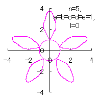
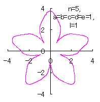
    If the (x, y) coordinate data of the shape of a flower are calculated by Eqs.(E1), (E2), (31), (27), (D3) and (D4), some examples of figures in the case of are obtained as shown below.

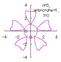
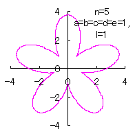
Fig.F1g  n=5, a=1, b=1, c=1,
d=1, e=1, l=0
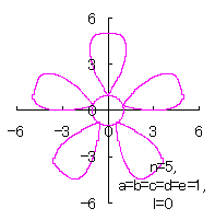
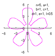
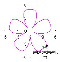
Fig.F1h  n=5, a=1, b=1, c=1,
d=1, e=1, l=0.5
Fig.F1i  n=5, a=1, b=1, c=1,
d=1, e=1, l=1
Fig.F1j  n=5, a=1, b=1, c=1,
d=1, e=1, l=1.5

     In purpose to calculate the numerical coordinates data of a flower by from Eqs.(E1), (E2), (31), (27), (D3) and (D4), a C++ program is given by C++ program_f2_independent_angle.
    By executing the C++ program, a text file named "C++ program_f2_independent_angle.txt" including the calculated data is produced.    Each interval of these data is divided by 'comma'.    After moving these calculated data into an excel file, we obtain a heart curve with the use of a graph wizard attached on the excel file.

Added in Oct. 16, 2012.


5.1.4 (ii)    The case 2

    The following two equations are proposed for replacing Eqs.(36) and (37).
          .                      (E3)
          ,                      (E4)
where the last term of Eq.(E4) is intended to move the origin to the bottom of the deformed circle.

    If the (x, y) coordinate data of the shape of a flower are calculated by Eqs.(E3), (E4), (31), (27), (D3) and (D4), some examples of figures in the case of are obtained as shown below.

Fig.F1k  n=5, a=1, b=1, c=1,
d=1, e=1, l=0
Fig.F1l  n=5, a=1, b=1, c=1,
d=1, e=1, l=0.5
Fig.F1m  n=5, a=1, b=1, c=1,
d=1, e=1, l=1

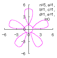
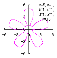
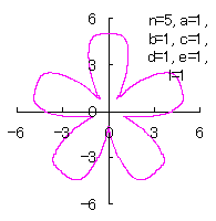
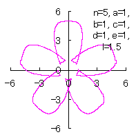
     In purpose to calculate the numerical coordinates data of a flower by from Eqs.(E3), (E4), (31), (27), (D3) and (D4), a C++ program is given by C++ program_f3_independent_angle.
    By executing the C++ program, a text file named "C++ program_f3_independent_angle.txt" including the calculated data is produced.    Each interval of these data is divided by 'comma'.    After moving these calculated data into an excel file, we obtain a heart curve with the use of a graph wizard attached on the excel file.

Added in Oct. 16, 2012.


5.1.4 (iii)    The case 3

     The following two equations are proposed for replacing Eqs.(36) and (37).
          .                      (E5)
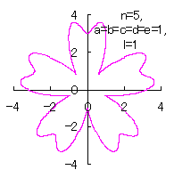
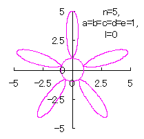
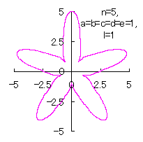
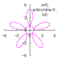
          ,                      (E6)
where the last term of Eq.(E6) is intended to move the origin to the bottom of the deformed circle.

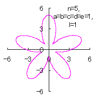
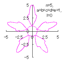
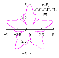
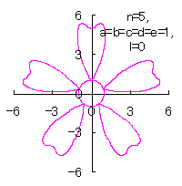
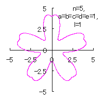
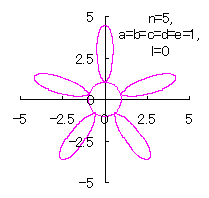
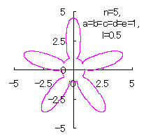
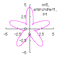
    If the (x, y) coordinate data of the shape of a flower are calculated by Eqs.(E5), (E6), (31), (27), (D3) and (D4), some examples of figures in the case of are obtained as shown below.

Fig.F1n  n=5, a=1, b=1, c=1,
d=1, e=1, l=0
Fig.F1o  n=5, a=1, b=1, c=1,
d=1, e=1, l=1

     In purpose to calculate the numerical coordinates data of a flower by from Eqs.(E5), (E6), (31), (27), (D3) and (D4), a C++ program is given by C++ program_f4_independent_angle.
    By executing the C++ program, a text file named "C++ program_f4_independent_angle.txt" including the calculated data is produced.    Each interval of these data is divided by 'comma'.    After moving these calculated data into an excel file, we obtain a heart curve with the use of a graph wizard attached on the excel file.

Added in Oct. 16, 2012.

5.1.4 (iv)    The case 4

    The following two equations are proposed for replacing Eqs.(36) and (37).
          .                      (E7)
          ,                      (E8)
where the last term of Eq.(E8) is intended to move the origin to the bottom of the deformed circle.

    If the (x, y) coordinate data of the shape of a flower are calculated by Eqs.(E7), (E8), (31), (27), (D3) and (D4), some examples of figures in the case of are obtained as shown below.

Fig.F1p  n=5, a=1, b=1, c=1,
d=1, e=1, l=0
Fig.F1q  n=5, a=1, b=1, c=1,
d=1, e=1, l=1

     In purpose to calculate the numerical coordinates data of a flower by from Eqs.(E7), (E8), (31), (27), (D3) and (D4), a C++ program is given by C++ program_f5_independent_angle.
    By executing the C++ program, a text file named "C++ program_f5_independent_angle.txt" including the calculated data is produced.    Each interval of these data is divided by 'comma'.    After moving these calculated data into an excel file, we obtain a heart curve with the use of a graph wizard attached on the excel file.

Added in Oct. 16, 2012.


5.1.4 (v)    The case 5


    The following two equations are proposed for replacing Eqs.(36) and (37).
          .                      (E9)
          ,                      (E10)
where the last term of Eq.(E10) is intended to move the origin to the bottom of the deformed circle.

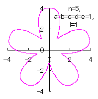
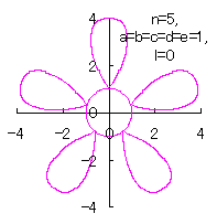
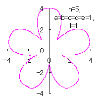
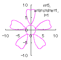
    If the (x, y) coordinate data of the shape of a flower are calculated by Eqs.(E9), (E10), (31), (27), (D3) and (D4), some examples of figures in the case of are obtained as shown below.


Fig.F1r  n=5, a=1, b=1, c=1,
d=1, e=1, l=0
Fig.F1s  n=5, a=1, b=1, c=1,
d=1, e=1, l=1

     In purpose to calculate the numerical coordinates data of a flower by from Eqs.(E9), (E10), (31), (27), (D3) and (D4), a C++ program is given by C++ program_f6_independent_angle.
    By executing the C++ program, a text file named "C++ program_f6_independent_angle.txt" including the calculated data is produced.    Each interval of these data is divided by 'comma'.    After moving these calculated data into an excel file, we obtain a heart curve with the use of a graph wizard attached on the excel file.

Added in Oct. 16, 2012.


5.1.4 (vi)    The case 6


     The following two equations are proposed for replacing Eqs.(36) and (37).
          .                      (E11)
          ,                      (E12)
where the last term of Eq.(E12) is intended to move the origin to the bottom of the deformed circle.

    If the (x, y) coordinate data of the shape of a flower are calculated by Eqs.(E11), (E12), (31), (27), (D3) and (D4), some examples of figures in the case of are obtained as shown below.


Fig.F1t  n=5, a=1, b=1, c=1,
d=1, e=1, l=0
Fig.F1u  n=5, a=1, b=1, c=1,
d=1, e=1, l=1

     In purpose to calculate the numerical coordinates data of a flower by from Eqs.(E11), (E12), (31), (27), (D3) and (D4), a C++ program is given by C++ program_f7_independent_angle.
    By executing the C++ program, a text file named "C++ program_f7_independent_angle.txt" including the calculated data is produced.    Each interval of these data is divided by 'comma'.    After moving these calculated data into an excel file, we obtain a heart curve with the use of a graph wizard attached on the excel file.

Added in Oct. 16, 2012.


5.1.4 (vii)    The case 7


    The following two equations are proposed for replacing Eqs.(36) and (37).
          .                      (E13)
          ,                      (E14)
where the last term of Eq.(E14) is intended to move the origin to the bottom of the deformed circle.

    If the (x, y) coordinate data of the shape of a flower are calculated by Eqs.(E13), (E14), (31), (27), (D3) and (D4), some examples of figures in the case of are obtained as shown below.


Fig.F1v  n=5, a=1, b=1, c=1,
d=1, e=1, l=0
Fig.F1w  n=5, a=1, b=1, c=1,
d=1, e=1, l=1

     In purpose to calculate the numerical coordinates data of a flower by from Eqs.(E13), (E14), (31), (27), (D3) and (D4), a C++ program is given by C++ program_f8_independent_angle.
    By executing the C++ program, a text file named "C++ program_f8_independent_angle.txt" including the calculated data is produced.    Each interval of these data is divided by 'comma'.    After moving these calculated data into an excel file, we obtain a heart curve with the use of a graph wizard attached on the excel file.

Added in Oct. 16, 2012.


5.2    The second deformation of a circle used as a petal


    We assume a deformed circle given in the followings in the orthogonal coordinates;
          .                      (38)
          ,                      (39)
where the last term in the parenthesis of Eq.(39) is intended to move the origin to the bottom of the deformed circle.

    As likely as in the previous section 5.1, Eq.(31) can be diverted as the moving radius.     Furthermore, As likely as in the previous section 5.1, Eqs.(32) and (33) is also diverted as the expression giving a shape of a flower in the orthogonal coordinates where indicates the phase angle around the shape of a flower and indicates the radius of a center circle surrounded by petals.

    As likely as in the previous section 5.1, we treat two cases of conversion of the phase angle from (that of a circle) to (that of the shape of a flower).
    One is the case of no overlap among the petals and another is the case of overlap among the petals.

5.2.1    In the case of no overlap among the petals of a flower

    As likely as in the previous section 5.1, Eq.(34) can be used as the equation of transformation from (the phase angle of a circle) to (the phase angle around the shape of a flower), where has to be replaced to .

    Calculating Eqs.(31) to (34), Eqs.(38) and (39), examples of shape of flower in the case of are obtained as shown below.


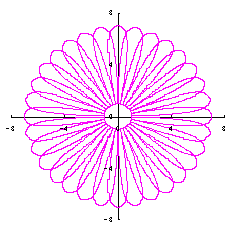
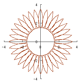
Fig.87 n=8, b=0.2, c=4, d=3, e=1
Fig.88a n=16, b=0, c=4, d=3, e=1
Fig.88b n=38, b=0, c=4, d=3, e=0
Fig.88c n=38, b=0, c=4, d=3, e=1
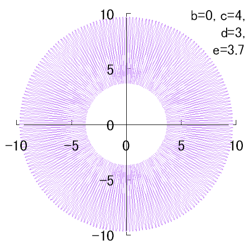
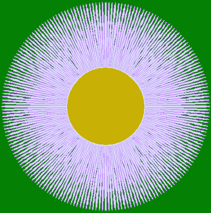
Fig.88d n=200, b=0, c=4, d=3, e=3.7

     When the above figures are painted, the following ones are drawn.    If clicked, an expanded line drawing appears.

Fig.87 n=8, b=0.2, c=4, d=3, e=1Fig.88a n=16, b=0, c=4, d=3, e=1Fig.88b n=38, b=0, c=4, d=3, e=0Fig.88c n=38, b=0, c=4, d=3, e=1Fig.88d


     In purpose to calculate the numerical coordinates data of a flower by Eqs.(31) to (34), Eqs.(38) and (39), a C++ program is given by C++ program_f1z.
    By executing the C++ program, a text file named "C++ program_f1z.txt" including the calculated data is produced.    Each interval of these data is divided by 'comma'.    After moving these calculated data into an excel file, we obtain a heart curve with the use of a graph wizard attached on the excel file.


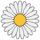
A part of the figures and the picture are added in May 14, 2013.


5.2.2    In the case of overlap among the petals of a flower

    As likely as in the previous section 5.1, Eq.(35-1) or (35-2) can be used as the equation of transformation from (the phase angle of a circle) to (the phase angle around the shape of a flower), where has to be replaced to .

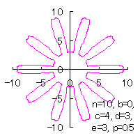
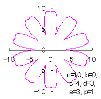
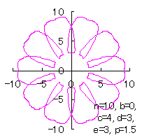
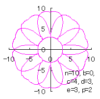
    Calculating Eqs.(31) to (33), either Eq.(35-1) or (35-2), Eqs.(38) and (39), examples of shape of flower in the case of are obtained as shown below.


Fig.89 n=5, b=0.2, c=4,
d=3, e=1, p=2
Fig.90 n=8, b=0.2, c=4,
d=3, e=1, p-2
Fig.91a n=16, b=0, c=4,
d=3, e=1, p=2
Fig.91b n=32, b=0, c=4,
d=3, e=1, p=2

>
Fig.92a n=10, b=0, c=4,
d=3, e=3,
p=0.5
Fig.92b n=10, b=0, c=4,
d=3, e=3,
p=1
Fig.92c n=10, b=0, c=4,
d=3, e=3,
p=1.5
Fig.92d n=10, b=0, c=4,
d=3, e=3,
p=2

Fig.92e n=10, b=0, c=4,
d=3, e=3,
p=3
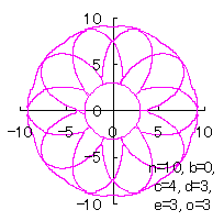
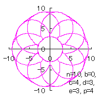
Fig.92f n=10, b=0, c=4,
d=3, e=3,
p=4

     When the above figures Figs.89 to 91b and Fig.92f are painted, they are drawn as in the folloings.    If the each of four figures in the middle is clicked, an expanded line drawing appears.

Fig.89 n=5, b=0.2, c=4, d=3, e=1Fig.89 n=5, b=0.2, c=4, d=3, e=1Fig.90 n=8, b=0.2, c=4, d=3, e=1Fig.91a n=16, b=0, c=4, d=3, e=1Fig.91b n=32, b=0, c=4, d=3, e=1Fig.92f n=10, b=0, c=4, d=3, e=3, p=4


     In purpose to calculate the numerical coordinates data of a flower by Eqs.(31) to (33), Eqs.(35-2), (38) and (39), a C++ program is given by C++ program_f2z.
    By executing the C++ program, a text file named "C++ program_f2z.txt" including the calculated data is produced.    Each interval of these data is divided by 'comma'.    After moving these calculated data into an excel file, we obtain a heart curve with the use of a graph wizard attached on the excel file.

edited in Mar. 15, 2009 & reviced in Sep. 15, 2012


5.2.3    In the case that each petal contacts with the center circle with an arbitral width of phase angle of its circle

     We can also use Eqs.(27), (31), (38) and (39).
    Moreover, we can consider the solution of this problem as followgs likely as in [3.2 Additional II] of the section 3.2.    So, we also use Eqs.(D3) and (D4).
    In calculating C program, we take the correction factor as an input variable, and then, we give the arbitral width of phase angle with which each petal contacts to the center circle.

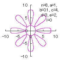
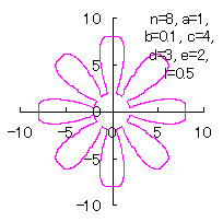
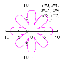
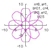
    The (x, y) coordinate data of the shape of a flower are calculated by Eqs.(27), (31), (38), (39), Eqs.(D3) and (D4),     Examples of such calculated shape of flower in the case of are shown below.


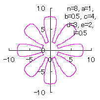
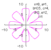
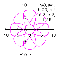
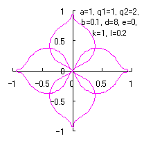
Fig.F2a  n=8, a=1, b=0.1, c=4,
d=3, e=2, l=0
Fig.F2b  n=8, a=1, b=0.1, c=4,
d=3, e=2, l=0.5
Fig.F2c  n=8, a=1, b=0.1, c=4,
d=3, e=2, l=1
Fig.F2d  n=8, a=1, b=0.1, c=4,
d=3, e=2, l=2.5

     In purpose to calculate the numerical coordinates data of a flower by Eqs.(27), (31), (38), (39), Eqs.(D3) and (D4), a C++ program is given by C++ program_fz_independent_angle.
    By executing the C++ program, a text file named "C++ program_fz_independent_angle.txt" including the calculated data is produced.    Each interval of these data is divided by 'comma'.    After moving these calculated data into an excel file, we obtain a heart curve with the use of a graph wizard attached on the excel file.

Added in Oct. 02, 2012.


5.2.4    The cases that the principal terms in Eqs.(38) and (39) are exchaneged mutually and/or the signs in Eqs.(38) and (39) are chaneged variously

     We treat several cases that the principal terms in Eqs.(38) and (39) are exchanged mutually and /or the signs contained in Eqs.(38) and (39) are chaneged variously while process of calculations is obeyed to that described in the section 5.2.3.


5.2.4 (i)    The case 1

     The following two equations are proposed for replacing Eqs.(38) and (39).
          .                      (F1)
          ,                      (F2)
where the last term of Eq.(F2) is intended to move the origin to the bottom of the deformed circle.

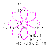
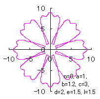
    If the (x, y) coordinate data of the shape of a flower are calculated by Eqs.(F1), (F2), (31), (27), (D3) and (D4), some examples of figures in the case of are obtained as shown below.

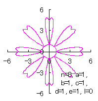
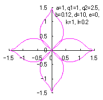
Fig.F2e  n=8, a=1, b=1, c=4,
d=3, e=2, l=1.5
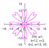
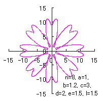
Fig.F2f  n=8, a=1, b=1.2, c=3,
d=2, e=1.5, l=1.5
Fig.F2g  n=8, a=1, b=2, c=4,
d=3, e=2, l=1

    When the above figure >Fig.F2f is painted, it is drawn as shown in the folloing.   If clicked, an expanded line drawing appears.

Fig.F2f n=8, a=1, b=1.2, c=3, d=2, e=1.5, l=1.5


     In purpose to calculate the numerical coordinates data of a flower by Eqs.(F1), (F2), (31), (27), (D3) and (D4), a C++ program is given by C++ program_fz2_independent_angle.
    By executing the C++ program, a text file named "C++ program_fz2_independent_angle.txt" including the calculated data is produced.    Each interval of these data is divided by 'comma'.    After moving these calculated data into an excel file, we obtain a heart curve with the use of a graph wizard attached on the excel file.

Added in Oct. 09, 2012.


5.2.4 (ii)    The case 2


     The following two equations are proposed for replacing Eqs.(38) and (39).
          .                      (F3)
          ,                      (F4)
where the last term of Eq.(F4) is intended to move the origin to the bottom of the deformed circle.

    If the (x, y) coordinate data of the shape of a flower are calculated by Eqs.(F3), (F4), (31), (27), (D3) and (D4), some examples of figures in the case of are obtained as shown below.


Fig.F2h  n=8, a=1, b=1, c=1,
d=1, e=1, l=0
Fig.F2i  n=8, a=1, b=1.2, c=3,
d=2, e=1.5, l=0
Fig.F2j  n=8, a=1, b=1.2, c=3,
d=2, e=1.5, l=1.5

     In purpose to calculate the numerical coordinates data of a flower by Eqs.(F3), (F4), (31), (27), (D3) and (D4), a C++ program is given by C++ program_fz3_independent_angle.
    By executing the C++ program, a text file named "C++ program_fz3_independent_angle.txt" including the calculated data is produced.    Each interval of these data is divided by 'comma'.    After moving these calculated data into an excel file, we obtain a heart curve with the use of a graph wizard attached on the excel file.

Added in Oct. 09, 2012.


5.2.4 (iii)    The case 3

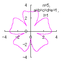
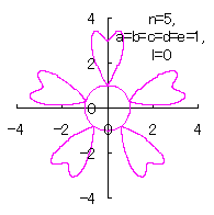
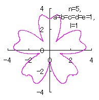
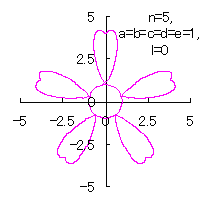
    The following two equations are proposed for replacing Eqs.(38) and (39).
          .                      (F5)
          ,                      (F6)
where the last term of Eq.(F6) is intended to move the origin to the bottom of the deformed circle.

    If the (x, y) coordinate data of the shape of a flower are calculated by Eqs.(F5), (F6), (31), (27), (D3) and (D4), some examples of figures in the case of are obtained as shown below.

Fig.F2k  n=8, a=1, b=1, c=1,
d=1, e=1, l=0
Fig.F2l  n=8, a=1, b=2, c=4,
d=3, e=2, l=0
Fig.F2m  n=8, a=1, b=2, c=4,
d=3, e=2, l=1

     In purpose to calculate the numerical coordinates data of a flower by Eqs.(F5), (F6), (31), (27), (D3) and (D4), a C++ program is given by C++ program_fz4_independent_angle.
    By executing the C++ program, a text file named "C++ program_fz4_independent_angle.txt" including the calculated data is produced.    Each interval of these data is divided by 'comma'.    After moving these calculated data into an excel file, we obtain a heart curve with the use of a graph wizard attached on the excel file.

Added in Oct. 09, 2012.


5.2.4 (iv)    The case 4

     The following two equations are proposed for replacing Eqs.(38) and (39).
          .                      (F7)
          ,                      (F8)
where the last term of Eq.(F8) is intended to move the origin to the bottom of the deformed circle.

    If the (x, y) coordinate data of the shape of a flower are calculated by Eqs.(F7), (F8), (31), (27), (D3) and (D4), some examples of figures in the case of are obtained as shown below.


Fig.F2n  n=5, a=1, b=1, c=1,
d=1, e=1, l=0
Fig.F2o  n=5, a=1, b=1, c=1,
d=1, e=1, l=1

     In purpose to calculate the numerical coordinates data of a flower by Eqs.(F7), (F8), (31), (27), (D3) and (D4), a C++ program is given by C++ program_fz5_independent_angle.

     By executing the C++ program, a text file named "C++ program_fz5_independent_angle.txt" including the calculated data is produced.    Each interval of these data is divided by 'comma'.    After moving these calculated data into an excel file, we obtain a heart curve with the use of a graph wizard attached on the excel file.

Added in Oct. 16, 2012.


5.2.4 (v)    The case 5


    The following two equations are proposed for replacing Eqs.(38) and (39).
          .                      (F9)
          ,                      (F10)
where the last term of Eq.(F10) is intended to move the origin to the bottom of the deformed circle.

    If the (x, y) coordinate data of the shape of a flower are calculated by Eqs.(F9), (F10), (31), (27), (D3) and (D4), some examples of figures in the case of are obtained as shown below.


Fig.F2p  n=5, a=1, b=1, c=1,
d=1, e=1, l=0
Fig.F2q  n=5, a=1, b=1, c=1,
d=1, e=1, l=1

     In purpose to calculate the numerical coordinates data of a flower by Eqs.(F9), (F10), (31), (27), (D3) and (D4), a C++ program is given by C++ program_fz6_independent_angle.
    By executing the C++ program, a text file named "C++ program_fz6_independent_angle.txt" including the calculated data is produced.    Each interval of these data is divided by 'comma'.    After moving these calculated data into an excel file, we obtain a heart curve with the use of a graph wizard attached on the excel file.

Added in Oct. 16, 2012.


5.2.4 (vi)    The case 6

    The following two equations are proposed for replacing Eqs.(38) and (39).
          .                      (F11)
          ,                      (F12)
where the last term of Eq.(F12) is intended to move the origin to the bottom of the deformed circle.

    If the (x, y) coordinate data of the shape of a flower are calculated by Eqs.(F11), (F12), (31), (27), (D3) and (D4), some examples of figures in the case of are obtained as shown below.


Fig.F2r  n=5, a=1, b=1, c=1,
d=1, e=1, l=0
Fig.F2s  n=5, a=1, b=1, c=1,
d=1, e=1, l=1

     In purpose to calculate the numerical coordinates data of a flower by Eqs.(F11), (F12), (31), (27), (D3) and (D4), a C++ program is given by C++ program_fz7_independent_angle.
    By executing the C++ program, a text file named "C++ program_fz7_independent_angle.txt" including the calculated data is produced.    Each interval of these data is divided by 'comma'.    After moving these calculated data into an excel file, we obtain a heart curve with the use of a graph wizard attached on the excel file.

Added in Oct. 16, 2012.


5.2.4 (vii)    The case 7

     The following two equations are proposed for replacing Eqs.(38) and (39).
          .                      (F13)
          ,                      (F14)
where the last term of Eq.(F14) is intended to move the origin to the bottom of the deformed circle.

    If the (x, y) coordinate data of the shape of a flower are calculated by Eqs.(F13), (F14), (31), (27), (D3) and (D4), some examples of figures in the case of are obtained as shown below.

Fig.F2t  n=5, a=1, b=1, c=1,
d=1, e=1, l=0
Fig.F2u  n=5, a=1, b=1, c=1,
d=1, e=1, l=0.5
Fig.F2v  n=5, a=1, b=1, c=1,
d=1, e=1, l=1

     In purpose to calculate the numerical coordinates data of a flower by Eqs.(F13), (F14), (31), (27), (D3) and (D4), a C++ program is given by C++ program_fz8_independent_angle.
    By executing the C++ program, a text file named "C++ program_fz8_independent_angle.txt" including the calculated data is produced.    Each interval of these data is divided by 'comma'.    After moving these calculated data into an excel file, we obtain a heart curve with the use of a graph wizard attached on the excel file.

Added in Oct. 16, 2012.


5.3    The third deformation of a circle used as a petal

     We assume a deformed circle given in the followings in the orthogonal coordinates;
          .                      (40)
          ,                      (41)
where the last term in the parenthesis of Eq.(41) is intended to move the origin to the bottom of the deformed circle.

    As likely as in the previous sections 5.1 and 5.2, Eq.(31) can be diverted as the moving radius.     Furthermore, As likely as in the previous sections 5.1 and 5.2, Eqs.(32) and (33) is also diverted as the expression giving a shape of a flower in the orthogonal coordinates, where indicates the phase angle around the shape of a flower and indicates the radius of a center circle surrounded by petals.

    As likely as in the previous sections 5.1 and 5.2, we treat two cases of conversion of the phase angle from (that of a circle) to (that of the shape of a flower).
    One is the case of no overlap among the petals and another is the case of overlap among the petals.

5.3.1    In the case of no overlap among the petals of a flower

    As likely as in the previous sections 5.1 and 5.2, Eq.(34) can be used as the equation of transformation from (the phase angle of a circle) to (the phase angle around the shape of a flower), where has to be replaced to .

    Calculating Eqs.(31) to (34), Eqs.(40) and (41), examples of shape of flower in the case of are obtained as shown below.

Fig.93 n=16, b=0.4, c=4, d=3, e=1
Fig.94 n=16, b=0.4, c=4.2, d=3, e=1
Fig.95 n=16, b=0.52, c=3.8, d=3, e=1

     When the above figures are painted, the following ones are drawn.    If clicked, an expanded line drawing appears.

Fig.93 n=16, b=0.4, c=4, d=3, e=1Fig.94 n=16, b=0.4, c=4.2, d=3, e=1Fig.95 n=16, b=0.52, c=3.8, d=3, e=1


     In purpose to calculate the numerical coordinates data of a flower by Eqs.(31) to (34), Eqs.(40) and (41), a C++ program is given by C++ program_f1zz.
    By executing the C++ program, a text file named "C++ program_f1zz.txt" including the calculated data is produced.    Each interval of these data is divided by 'comma'.    After moving these calculated data into an excel file, we obtain a heart curve with the use of a graph wizard attached on the excel file.


5.3.2    In the case of overlap among the petals of a flower

    As likely as in the previous sections 5.1 and 5.2, either Eq.(35-1) or (35-2) can be used as the equation of transformation from (the phase angle of a circle) to (the phase angle around the shape of a flower), where has to be replaced to .

    Calculating Eqs.(31) to (33), either Eq.(35-1) or (35-2), Eqs.(40) and (41), examples of shape of flower in the case of are obtained as shown below.


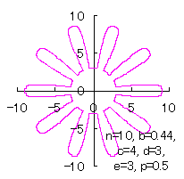
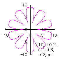
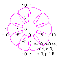
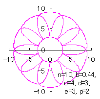
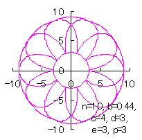
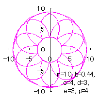
Fig.96a n=16, b=0.44,
c=4, d=3, e=1, p=2
Fig.96b n=32, b=0.44,
c=4, d=3, e=1, p=2
Fig.97a n=16, b=0.44,
c=4, d=3, e=3,
p=0.5
Fig.97b n=32, b=0.44,
c=4, d=3, e=3,
p=1

Fig.97c n=16, b=0.44,
c=4, d=3, e=3,
p=1.5
Fig.97d n=32, b=0.44,
c=4, d=3, e=3,
p=2
Fig.97e n=16, b=0.44,
c=4, d=3, e=3,
p=3
Fig.97f n=32, b=0.44,
c=4, d=3, e=3,
p=4

     When the above figures Figs.96a and b are painted, they are drawn as in the folloings.    If the each of four figures in the left side is clicked, an expanded line drawing appears.

Fig.96a n=16, b=0.44, c=4, d=3, e=1Fig.96b n=32, b=0.44, c=4, d=3, e=1Fig.97f n=10, b=0.44, c=4, d=3, e=3, p=4


     In purpose to calculate the numerical coordinates data of a flower by Eqs.(31) to (33), Eqs.(35-2), (40) and (41), a C++ program is given by C++ program_f2zz.
     By executing the C++ program, a text file named "C++ program_f2zz.txt" including the calculated data is produced.    Each interval of these data is divided by 'comma'.    After moving these calculated data into an excel file, we obtain a heart curve with the use of a graph wizard attached on the excel file.

edited in Mar. 15, 2009 & reviced in Sep. 16, 2012


5.3.3    In the case that each petal contacts with the center circle with an arbitral width of phase angle of its circle

    We can also use Eqs.(27), (31), (40) and (41).
    Moreover, we can consider the solution of this problem as followgs likely as in [3.2 Additional II] of the section 3.2.    So, we also use Eqs.(D3) and (D4).
    In calculating C program, we take the correction factor as an input variable, and then, we give the arbitral width of phase angle with which each petal contacts to the center circle.

    The (x, y) coordinate data of the shape of a flower are calculated by Eqs.(27), (31), (40), (41), Eqs.(D3) and (D4),     Examples of such calculated shape of flower in the case of are shown below.

Fig.F3a  n=8, a=1, b=0.5, c=4,
d=3, e=2, l=0
Fig.F3b  n=8, a=1, b=0.5, c=4,
d=3, e=2, l=0.5
Fig.F3c  n=8, a=1, b=0.5, c=4,
d=3, e=2, l=1
Fig.F3d  n=8, a=1, b=0.5, c=4,
d=3, e=2, l=2.5

     In purpose to calculate the numerical coordinates data of a flower by Eqs.(27), (31), (40), (41), Eqs.(D3) and (D4), a C++ program is given by C++ program_fzz_independent_angle.
    By executing the C++ program, a text file named "C++ program_fzz_independent_angle.txt" including the calculated data is produced.    Each interval of these data is divided by 'comma'.    After moving these calculated data into an excel file, we obtain a heart curve with the use of a graph wizard attached on the excel file.

Added in Oct. 02, 2012.


5.3.4    The cases that the principal terms in Eqs.(40) and (41) are exchaneged mutually and/or the signs in Eqs.(40) and (41) are chaneged variously

     We treat several cases that the principal terms in Eqs.(40) and (41) are exchanged mutually and /or the signs contained in Eqs.(40) and (41) are chaneged variously while process of calculations is obeyed to that described in the section 5.3.3.

5.3.4 (i)    The case 1

    The following two equations are proposed for replacing Eqs.(40) and (41).
          .                      (G1)
          ,                      (G2)
where the last term of Eq.(G2) is intended to move the origin to the bottom of the deformed circle.

    If the (x, y) coordinate data of the shape of a flower are calculated by Eqs.(27), (31), (G1), (G2), (D3) and (D4), some examples of figures in the case of are obtained as shown below.


Fig.F3e  n=5, a=1, b=1, c=1,
d=1, e=1, l=0
Fig.F3f  n=5, a=1, b=1, c=1,
d=1, e=1, l=1

     In purpose to calculate the numerical coordinates data of a flower by Eqs.(27), (31), (G1), (G2), (D3) and (D4), a C++ program is given by C++ program_fzz2_independent_angle.
    By executing the C++ program, a text file named "C++ program_fzz2_independent_angle.txt" including the calculated data is produced.    Each interval of these data is divided by 'comma'.    After moving these calculated data into an excel file, we obtain a heart curve with the use of a graph wizard attached on the excel file.

Added in Oct. 16, 2012.


5.3.4 (ii)    The case 2


    The following two equations are proposed for replacing Eqs.(40) and (41).
          .                      (G3)
          ,                      (G4)
where the last term of Eq.(G4) is intended to move the origin to the bottom of the deformed circle.

    If the (x, y) coordinate data of the shape of a flower are calculated by Eqs.(27), (31), (G3), (G4), (D3) and (D4), some examples of figures in the case of are obtained as shown below.

Fig.F3g  n=5, a=1, b=1, c=1,
d=3, e=2, l=0
Fig.F3h  n=5, a=1, b=1, c=1,
d=1, e=1, l=1

     In purpose to calculate the numerical coordinates data of a flower by Eqs.(27), (31), (G3), (G4), (D3) and (D4), a C++ program is given by C++ program_fzz3_independent_angle.
    By executing the C++ program, a text file named "C++ program_fzz3_independent_angle.txt" including the calculated data is produced.    Each interval of these data is divided by 'comma'.    After moving these calculated data into an excel file, we obtain a heart curve with the use of a graph wizard attached on the excel file.

Added in Oct. 16, 2012.


5.3.4 (iii)    The case 3

     The following two equations are proposed for replacing Eqs.(40) and (41).
          .                      (G5)
          ,                      (G6)
where the last term of Eq.(G6) is intended to move the origin to the bottom of the deformed circle.

    If the (x, y) coordinate data of the shape of a flower are calculated by Eqs.(27), (31), (G5), (G6), (D3) and (D4), some examples of figures in the case of are obtained as shown below.


Fig.F3i  n=5, a=1, b=1, c=1,
d=3, e=2, l=0
Fig.F3j  n=5, a=1, b=1, c=1,
d=1, e=1, l=1

     In purpose to calculate the numerical coordinates data of a flower by Eqs.(27), (31), (G5), (G6), (D3) and (D4), a C++ program is given by C++ program_fzz4_independent_angle.
    By executing the C++ program, a text file named "C++ program_fzz4_independent_angle.txt" including the calculated data is produced.    Each interval of these data is divided by 'comma'.    After moving these calculated data into an excel file, we obtain a heart curve with the use of a graph wizard attached on the excel file.

Added in Oct. 16, 2012.


5.3.4 (iv)    The case 4


    The following two equations are proposed for replacing Eqs.(40) and (41).
          .                      (G7)
          ,                      (G8)
where the last term of Eq.(G8) is intended to move the origin to the bottom of the deformed circle.

    If the (x, y) coordinate data of the shape of a flower are calculated by Eqs.(27), (31), (G7), (G8), (D3) and (D4), some examples of figures in the case of are obtained as shown below.

Fig.F3k  n=5, a=1, b=1, c=1,
d=3, e=2, l=0
Fig.F3l  n=5, a=1, b=1, c=1,
d=1, e=1, l=1

     In purpose to calculate the numerical coordinates data of a flower by Eqs.(27), (31), (G7), (G8), (D3) and (D4), a C++ program is given by C++ program_fzz5_independent_angle.
    By executing the C++ program, a text file named "C++ program_fzz5_independent_angle.txt" including the calculated data is produced.    Each interval of these data is divided by 'comma'.    After moving these calculated data into an excel file, we obtain a heart curve with the use of a graph wizard attached on the excel file.

Added in Oct. 16, 2012.


5.3.4 (v)    The case 5

     The following two equations are proposed for replacing Eqs.(40) and (41).
          .                      (G9)
          ,                      (G10)
where the last term of Eq.(G10) is intended to move the origin to the bottom of the deformed circle.

    If the (x, y) coordinate data of the shape of a flower are calculated by Eqs.(27), (31), (G9), (G10), (D3) and (D4), some examples of figures in the case of are obtained as shown below.


Fig.F3m  n=5, a=1, b=1, c=1,
d=3, e=2, l=0
Fig.F3n  n=5, a=1, b=1, c=1,
d=1, e=1, l=1

     In purpose to calculate the numerical coordinates data of a flower by Eqs.(27), (31), (G9), (G10), (D3) and (D4), a C++ program is given by C++ program_fzz6_independent_angle.
    By executing the C++ program, a text file named "C++ program_fzz6_independent_angle.txt" including the calculated data is produced.    Each interval of these data is divided by 'comma'.    After moving these calculated data into an excel file, we obtain a heart curve with the use of a graph wizard attached on the excel file.

Added in Oct. 16, 2012.


5.3.4 (vi)    The case 6

     The following two equations are proposed for replacing Eqs.(40) and (41).
          .                      (G11)
          ,                      (G12)
where the last term of Eq.(G12) is intended to move the origin to the bottom of the deformed circle.

    If the (x, y) coordinate data of the shape of a flower are calculated by Eqs.(27), (31), (G11), (G12), (D3) and (D4), some examples of figures in the case of are obtained as shown below.


Fig.F3o  n=5, a=1, b=1, c=1,
d=3, e=2, l=0
Fig.F3p  n=5, a=1, b=1, c=1,
d=1, e=1, l=1

     In purpose to calculate the numerical coordinates data of a flower by Eqs.(27), (31), (G11), (G12), (D3) and (D4), a C++ program is given by C++ program_fzz7_independent_angle.
     By executing the C++ program, a text file named "C++ program_fzz7_independent_angle.txt" including the calculated data is produced.    Each interval of these data is divided by 'comma'.    After moving these calculated data into an excel file, we obtain a heart curve with the use of a graph wizard attached on the excel file.

Added in Oct. 16, 2012.


5.3.4 (vii)    The case 7

     The following two equations are proposed for replacing Eqs.(40) and (41).
          .                      (G13)
          ,                      (G14)
where the last term of Eq.(G14) is intended to move the origin to the bottom of the deformed circle.

     If the (x, y) coordinate data of the shape of a flower are calculated by Eqs.(27), (31), (G13), (G14), (D3) and (D4), some examples of figures in the case of are obtained as shown below.


Fig.F3q  n=5, a=1, b=1, c=1,
d=3, e=2, l=0
Fig.F3r  n=5, a=1, b=1, c=1,
d=1, e=1, l=1

     In purpose to calculate the numerical coordinates data of a flower by Eqs.(27), (31), (G13), (G14), (D3) and (D4), a C++ program is given by C++ program_fzz8_independent_angle.

     By executing the C++ program, a text file named "C++ program_fzz8_independent_angle.txt" including the calculated data is produced.    Each interval of these data is divided by 'comma'.    After moving these calculated data into an excel file, we obtain a heart curve with the use of a graph wizard attached on the excel file.

Added in Oct. 16, 2012.


6.    Method to draw to set independently both of the phase angles of each petal and a center circle underlying each other

     In the previous sections, a flower has been configured with the common phase angle of a center circle and its underlying each petal.    In this manner, the width of the petal cannot be extended beyond the area of a predetermined phase angle of the center circle underlying.
    Therefore, although the fundamental configuration of the petal is also performed as above, going back to the origin, we try the design of a flower again from the beginning in such the manner as we set independently both of the phase angles of each petal and a center circle underlying each other.
     The design of a flower will be performed starting from using the circle originated petals and then will be also performed with the use of the petals originated from heart curves if we can afford,


Fig.98b  Petal
Fig.98a  Original circle
6.1   The case with the use of circle originated petals

     The petal as shown in Fig.98b is created by sharpened the bottom of the circle as shown in Fig.98a.    The equation of the circle in Fig.98a is described as
          ,                      (42)
where and is described as
          ,                      (43)
where .


Fig.99  Conversion of the phase angle from to

     In the next, in order that the bottom of the circle is reformed into a petal curve with a corner having the desired angle (as seen in Fig.98b), we converse the phase angle of the circle into the newly defined phase angle of the petal curve linearly as shown in Fig.99.
    A conversion equation which satisfies the above mention may be given as
          .                      (44)
    If we substitute Eq.(43) into Eq.(44), the conversion equation from to is obtained as
          .                      (45)
     The orthogonal coordinate expression of the petal may be written as the following two equations;
          ,                      (46)
and
          .                      (47)

    We will arrange such the obtained petal curve around a center circle for making a flower graphics.    If numbers of petals are arranged, we assume that the reference angle of the bottom of each petal is taken as the angle going around a flower divided by as given in the following equation;
          .                      (48)
    If you want to change the width of the petal, then the angle of the bottom of the petal is multiplied by the rate of deformation, and such a deformed angle may be agqin defined as the angle of the bottom of the petal where 0 < .
          .                      (48b)

    When the number is assigned to each of petals, the phase angle of -th number's of petal is expressed in the following equation into which the angle is added to .
          .                      (49)

    Though numbers of petals around a center circle is described above, we consider the flower grapics in several way of petal arrangement in the following each subsection.


6.1.1    In the same case as in the previous sections in which common phase angle is applied to both of the each petal and the center circle underlying   (reference for comparison)

     In this case, the entire shape of a flower is expressed in the following two equations which are the same to Eqs.(6) and (7) in the section 2.1.
          ,                      (50)
          .                      (51)


Fig.100 n=5, k=1, c=1

     Calculating Eq.(42), either Eq.(48) or Eq.(48b), Eqs.(49), (50) and (51), an example of shape of flower in the case of is obtained as shown in Fig.100.

In purpose to calculate the numerical coordinates data of a flower by Eqs.(42), (48b), (49), (50) and (51), a C++ program is given by C++ program_circle_flower_A.
    By executing the C++ program, a text file named "flower_curve_A.txt" including the calculated data is produced.    Each interval of these data is divided by 'comma'.    After moving these calculated data into an excel file, we obtain a heart curve with the use of a graph wizard attached on the excel file.


6.1.2   In the case that the phase angle of a center circle is set independently on the phase angle of each petal

     According to how each petal contacts with the center circle, we will compose a flower graphics as divided into following three cases.

6.1.2 (i)   In the case that each petal contacts with the center circle at one point

    In this case, as the phase angle of the centercircle takes the fixed value at the contact point with each petal, then, the following two equations are used instead of Eqs.(50) and (51).   nbsp;Herein, the reason why the term of exists in this equation is because the central phase of the first () petal is situated at of the phase of the center circle, and then, the count of the phase of the each petal starts from this phase .    The other equations used are the same ones given in the previous subsection 6.1.1.    In addition, there may be a need to draw a separate center circle connecting each point of each petal in contact with the center circle.
          ,                      (52)
          ,                      (53)
where is the radius of the center circle.


Fig.101 n=5, k=1, c=1

     Calculating Eqs.(42), (48) or (48b), (49), (52) and (53), an example of shape of flower in the case of is obtained as shown in Fig.101.

In purpose to calculate the numerical coordinates data of a flower by Eqs.(42), (48b), (49), (52) and (53), a C++ program is given by C++ program_circle_flower_B.
    By executing the C++ program, a text file named "flower_curve_B.txt" including the calculated data is produced.    Each interval of these data is divided by 'comma'.    After moving these calculated data into an excel file, we obtain a heart curve with the use of a graph wizard attached on the excel file.


6.1.2 (ii)   In the case that each petal contacts with the center circle with an arbitral width of phase angle of its circle

     If we take as an arbitral width of phase angle with which each petal contacts with the center circle, the phase angle of the center circle is discribed as , and then, it depends on .
    Accordingly, the following two equations are used instead of Eqs.(52) and (53).    The other equations used are the same ones given in the previous subsections.    In addition, there may be a need to draw a separate center circle connecting each neighbouring petals in the contact region.
          ,                      (54)
          ,                      (55)
where is the radius of the center circle.
    Calculating Eq.(42), either Eq.(48) or Eq.(48b), Eqs.(49), (54) and (55), an example of shape of flower in the case of is obtained as shown in Figs.102a to f.


Fig.102a n=5, k=1, l=0.3, c=1
Fig.102b n=5, k=1, l=1, c=1
Fig.102c n=5, k=1, l=1.5, c=1
Fig.102d n=5, k=1, l=2, c=1

Fig.102g
Fig.102e n=8, k=1, l=0.3, c=1.5
Fig.102f n=10, k=1, l=2.5, c=1
Fig.102g n=5, k=2.4, l=0.1, c=0.6

In purpose to calculate the numerical coordinates data of a flower by Eqs.(42), (48b), (49), (54) and (55), a C++ program is given by C++ program_circle_flower_C.
    By executing the C++ program, a text file named "flower_curve_C.txt" including the calculated data is produced.    Each interval of these data is divided by 'comma'.    After moving these calculated data into an excel file, we obtain a heart curve with the use of a graph wizard attached on the excel file.


6.1.2 (iii)   In the case to sharpen the tip of the petal treated in the subsection 6.1.2 (ii)


>     It is needed only that Eq.(42) is exchanged to the following equation for an example.    The other equations used are the same ones given in the previous subsections.    In addition, there may be a need to draw a separate center circle connecting each neighbouring petals in the contact region.
          .                      (56-1)

    Calculating Eqs.(56-1), either Eq.(48) or Eq.(48b), Eqs.(49), (54) and (55), examples of shape of flower in the case of are obtained as shown in Figs.103a, 103b, 103c and 103d, where magnification factor "l" of some angular range will be explained in the calculation program described below.


(If clicked, an expanded
line drawing appears.)
Fig.104 n=32, b=1, k=5.3, l=0.3, c=1.5
Fig.103a n=5, b=1, k=1, l=0.3, c=1
Fig.104b n=32, b=1, k=5.3, l=0.3, c=1.5

(If clicked, an expanded
line drawing appears.)
Fig.103c n=3, b=0.7, k=1.1, c=l=0
Fig.103d n=3, b=1, k=2, c=l=0

     In purpose to calculate the numerical coordinates data of a flower by Eqs.(56-1), (48b), (49), (54) and (55), a C++ program is given by C++ program_circle_flower_D.
    By executing the C++ program, a text file named "flower_curve_D.txt" including the calculated data is produced.    Each interval of these data is divided by 'comma'.    After moving these calculated data into an excel file, we obtain a heart curve with the use of a graph wizard attached on the excel file.

July 09, 2012 & Sep 09, 2012

6.1.2 (iv)   In the case to sharpen the tip of the petal treated in the subsection 6.1.2 (ii)...(part 2)


     Eq.(56-1) given in the previous section 6.1.2 (iii) is tried to be changed in the following.
          ,                      (56-2)

    Calculating Eqs.(56-2), either Eq.(48) or Eq.(48b), Eqs.(49), (54) and (55), example of shape of flower in the case of is obtained as shown in Fig.104, where magnification factor "l" of some angular range will be explained in the calculation program described below.


(If clicked, an expanded
line drawing appears.)
Fig.104 n=3, b=0.7, k=1.1 c=l=0

     In purpose to calculate the numerical coordinates data of a flower by Eqs.(56-2), (48b), (49), (54) and (55), a C++ program is given by C++ program_circle_flower_D2.
    By executing the C++ program, a text file named "flower_curve_D2.txt" including the calculated data is produced.    Each interval of these data is divided by 'comma'.    After moving these calculated data into an excel file, we obtain a heart curve with the use of a graph wizard attached on the excel file.

Sep 09, 2012

6.2   The case to configure the petals from cardioid

     There are two methods of the method 1 and 2 described in Section 2 and 3 respectively to convert the underlying heart curve in the form of a petal from cardioid.    We will design a flower graphics according to the each method in case by case as below.


6.2.1   In the case with the use of the method 1 described in Section 2

Fig.105b  Heart curve
to be the source of petal
Fig.105a  The original Cardioid

     We will treat a flower graphics along to "Method 1" described in Section 2.    Unlike Section 2, we set independently of each other between the phase angle of petal and that of a center circle underlying.    Therefore, though the following description may overlap with Section 2, its description is intended to be re-recorded for clarity.

    The original Cardioid is shown in Fig,105a, and the heart curve, which is produced from this original Cardioid by the method 1 as described in the page of "heart curves II", is shown in Fig.105b.    We intend to form a shape of flower by arranging heart curves around a center circle as petals of a flower.
    The equations obtained in the page of "heart curves II" and used also in this section are the following ones;
          ,                      (57)
where .

          ,                      (58)
where .

    The newly defined phase angle of the Cardioid after the replacement of the coordinate origin, which is shown in Fig.105a, is written as
          ,                      (59)
where .


Fig.106   Conversion of the phase
angle from into


    In the next, in order that the bottom of the Cardioid is reformed into a heart curve with a corner having the desired angle (as seen in Fig.105b), we converse the phase angle of the Cardioid into the newly defined phase angle of the heart curve linearly as shown in Fig.106.    A conversion equation which satisfies the above mention may be given as
          .                      (60)
    If we substitute Eq.(59) into Eq.(60), the conversion equation from to is obtained as

          .                      (61)
    The orthogonal coordinate expression of the heart curve may be written as the following two equations;
          .                      (62)
          .                      (63)
    In order to broaden the variety in the form of a petal, we introduce the ratio of expansion in the y direction, and we rewrite Eq.(63) into the following equation with the use of .
          .                      (63b)
    In the next, we express the heart curve in the polar coordinates again.    In this case, the moving radius and the phase angle are given by the followings;
          ,                      (64)
          ,                      (65)

    We will arrange such the obtained heart curves as petals of a flower around a center circle of radius .    If numbers of petals are arranged, we assume that the reference angle of the bottom of each petal is taken as the angle going around a flower divided by as given in the following equation;
          .                      (66)
    If the number is assigned to the each of petals, the phase angle of -th number's of petal is expressed in the following equation into which the angle described in Eq.(65) is added to .
          .                      (67)

Fig.107  Width of phase angle with which
each petal contacts with the center circle
and the phase of the center circle

     On theother hand, if we take as an arbitral width of phase angle with which each petal contacts with the center circle, the phase angle of the center circle in contact with the -th petal is described as , and then, it depends on .
          ,                      (68)
where and is the maximum and minimum values of the phase angle [which is defined in Fig.105a and appears also in Eq.(57)] of Cardioid of the underlying one of each petal.    Herein, the reason why the term of exists in this equation is because the central phase of the first () petal is situated at of the phase of the center circle, and then, the count of the phase of the each petal starts from this phase .

    Thus, the entire shape of a flower is expressed in the following two equations which are in the same manner as Eqs.(54) and (55).
          .                      (69)
          .                      (70)

    Calculating Eqs.(57) to (70), examples of shape of flower in the case of are obtained as shown in figures from Figs.108 to 114.


Fig.108 n=5, b=1, c=0, k=1, l=0
Fig.109 n=5, b=1, c=1, k=1.5, l=0
Fig.110 n=5, b=1, c=1, k=1, l=0.3
Fig.111 n=5, b=0.5, c=1, k=1, l=0.3

Fig.112 n=5, b=1, c=1, k=1, l=0.5
Fig.113 n=5, b=1, c=1, k=1, l=1
Fig.114 n=5, b=1, c=1, k=1, l=1.5

    In purpose to calculate the numerical coordinates data of a flower by Eqs.(57) to (70), a C++ program is given by C++ program_flower_g.
    By executing the C++ program, a text file named "flower_g.txt" including the calculated data is produced.    Each interval of these data is divided by 'comma'.    After moving these calculated data into an excel file, we obtain a heart curve with the use of a graph wizard attached on the excel file.

July 14, 2012

6.2.2   In the case with the use of the method 2 described in the section 3

     We will treat a flower graphics along to "Method 2" described in Section 3.    Unlike Section 3, we set independently of each other between the phase angle of petal and that of a center circle underlying.    Therefore, though the following discription may overlap with Section 3, its discription is intended to be re-recorded for clarity.

    The original Cardioid is shown in Fig,115a, and the heart curve, which is produced from this original Cardioid by the method 2 as described in the page of "heart curves II", is shown in Fig.115b.    We intend to form a shape of flower by arranging heart curves around a center circle as petals of a flower.
    The outline of the method 2 is to convert the phase angle such that the bottom of the Cardioid becomes to sharpen.    Specifically, the phase angle of the Cardioid (as seen in Fig.115a) is converted into (as seen in Fig.115b) the phase angle of the heart curve according to the conversion rule shown in Fig.115c.
    As an example of the conversion rule, we assume the folloing conversion equation with the use of the combination of the square root and the linear functions as discribed in Eqs.(9a) and (9b) in the page "heart curves II".
          ,                      (71)
where is the positive real constant displaying the strength of conversion.    It has to be taken in account that has not periodicity and is applied only in the range of as shown in Fig.115c.

Fig.115a  Original Cardioid
Fig.115b  Heart curve
Fig.115c  Conversion of the phase angle
from
into

     Thus, the phase angle is converted as that the bottom of the cardioid becomes to sharpen.
    Moreover, in order to obtain beautiful shape of heart figure, both of the coefficient for the reformation and the compression coefficient in the length direction are included in the following conversion equations in the (x, y) coordinates.
          ,                        (72a)
and
          ,                      (72b)
where
          .                      (73)
    The origin point in Fig.115b is needed to be moved to the bottom of the heart curve.    Although Eq.(72a) is not varied in such a displacement, Eq.(72b) should be varied in the following equation.
          .                      (74)
    After the displacement of the origin point, the moving radius and the phase angle , which is described as "ff" in the C program below, are written in the following equations;
          .                      (75)
          .                      (76)
    To change the width of the heart curve and, as the result, to change the angle of the bottom of the heart curve, the rate of deformation (where 0 < ) is multiplied to the phase of Eq.(76), and the phase is re-defined as the following equation.    Herein, the reason why the term of exists in this equation is because the shape of this heart curve is symmetrical to the phase angle .
          .                      (76b)

   We will arrange such the obtained heart curves as petals of a flower around a center circle of radius .    If numbers of petals are arranged and if the number is assigned to the each of petals, the phase angle of -th number's of petal is expressed in the following equation into which the angle described in Eq.(76b) is added to .
          .                      (77)

Fig.116  Width of phase angle with which
each petal contacts with the center circle
and the phase of the center circle

    On the other hand, if we take as an arbitral width of phase angle with which each petal contacts with the center circle, the phase angle of the center circle in contact with the -th petal is depends on as likely as in the subsection 6.2.1.
          ,                      (78)
where and is the maximum and minimum values of the phase angle (which is defined in Fig.115b) of a heart curve of the underlying each petal.    Herein, the reason why the term of exists in this equation is because the central phase of the first () petal is situated at of the phase of the center circle, and then, the count of the phase of the each petal starts from this phase .

     Thus, the entire shape of a flower is expressed in the following two equations which are in the same manner as Eqs.(69) and (70).
          .                      (79)
          .                      (80)

    Calculating Eqs.(71) to (80), examples of shape of flower in the case of are obtained as shown in figures from Figs.117 to 126.


Fig.117 n=5, b=2, c=0, d=1,
e=0, k=1, l=0
Fig.118 n=5, b=2, c=0, d=1,
e=1, k=1, l=0
Fig.119 n=5, b=2, c=0, d=1,
e=1, k=1, l=0.5
Fig.120 n=5, b=2, c=0, d=1,
e=1, k=1, l=1

Fig.121 n=5, b=2, c=0, d=1,
e=1, k=1, l=1.5
Fig.122 n=5, b=2, c=0, d=1,
e=1, k=1.5, l=0.5
Fig.123 n=5, b=2, c=0, d=1,
e=1, k=2, l=0.5
Fig.124 n=5, b=2, c=0, d=1,
e=1, k=2, l=0

Fig.125 n=5, b=2,
c=0, d=1, e=1, k=2, l=1
Fig.126 n=5, b=0.5, c=1, d=1,
e=1, k=2, l=0.5
Fig.127 n=5, b=1, c=0, d=1,
e=0.5, k=1, l=0.3
Fig.128 n=5, b=1, c=0, d=1,
e=0.5, k=0.7, l=1

Fig.129 n=5, b=1, c=0,
d=1, e=0.2, k=0.8, l=1
Fig.130 n=5, b=1, c=-0.2,
d=1, e=0.2, k=0.8, l=1
Fig.131 n=5, b=1, c=0.2,
d=1, e=0.2, k=0.8, l=1
Fig.132a n=5, b=2.5, c=0.65,
d=1, e=0.2, k=1.5, l=1

Fig.132b n=5, b=3, c=0.8,
d=1.5, e=0.1, k=1.5, l=1
Fig.132c n=5, b=2.8, c=0.8,
d=1.5, e=0.2, k=1.8, l=1
Fig.132d n=5, b=1.8, c=0.8,
d=1.5, e=0.2, k=0.6, l=1

     When Figs.127, 128 and 132d are painted, the following figures are drawn.    If clicked, an expanded line drawing appears.

Fig.127 n=5, b=1, c=0, d=1, e=0.5, k=1, l=0.3Fig.128 n=5, b=1, c=0, d=1, e=0.5, k=0.7, l=1Fig.132d

    In purpose to calculate the numerical coordinates data of a flower by Eqs.(71) to (80), a C++ program is given by C++ program_flower_h.
    By executing the C++ program, a text file named "flower_h.txt" including the calculated data is produced.    Each interval of these data is divided by 'comma'.    After moving these calculated data into an excel file, we obtain a heart curve with the use of a graph wizard attached on the excel file.

July 18, 2012 and May 14, 2013.

6.2.3   Deformation of the previous subsection 6.2.2


     To simulate the cherry blossom of varieties of "Prunus yedoensis" has been recognized to be impossible in any method mentioned above.    In this time, it is found to become possible by using Eq.(81) in the following subsection 6.2.3 (i) instead of Eq.(72a) in section 6.2.2.    It is for the first time to use with which the derivatives of the curve of a single petal becomes discontinuous.
    Subsequently, in each time of changing the insertion place of in the equation expressing a single petal, we will treat flower graphics in added subsection.

6.2.3 (i)   Deformation I of the previous section 6.2.2

    The following equation is replaced to Eq.(72a) in the previous section 6.2.2.
          .                      (81)

    Calculating Eq.(71), Eqs.(72b) to (80) and Eq.(81), examples of shape of flower in the case of are obtained as shown in figures from Figs.133 and 134.


Fig.133a n=5, b=1, c=0.2,
d=1.25, e=0.2, k=0.75, l=1
Fig.133b n=5, b=1, c=0.2,
d=1.3, e=0.2, k=0.75, l=1
Fig.134 n=32, b=3, c=0.2,
d=3, e=2.3, k=1.2, l=0.8

     When the above figures are painted, the following ones are drawn.    If clicked, a line drawing appears.

Fig.133aFig.133bFig.134


     In purpose to calculate the numerical coordinates data of a flower by Eq.(71), Eqs.(72b) to (80) and Eq.(81a), a C++ program is given by C++ program_flower_i.
    By executing the C++ program, a text file named "flower_i.txt" including the calculated data is produced.    Each interval of these data is divided by 'comma'.    After moving these calculated data into an excel file, we obtain a heart curve with the use of a graph wizard attached on the excel file.

July 18, 2012 and May 09, 2013.

6.2.3 (ii)   Deformation II of the previous section 6.2.2

     The following equations are replaced to Eqs.(72a) and (72b) respectively in the previous section 6.2.2.
          .                      (82a)
          .                      (82b)

    Calculating Eq.(71), Eqs.(73) to (80), Eqs.(82a) and (82b), examples of shape of flower in the case of are obtained as shown below.

Fig.135a n=5, b=1, c=0.2,
d=1, e=0.3, k=0.7, l=1
Fig.135b n=5, b=1, c=0.2,
d=1, e=0.3, k=1, l=1
Fig.135c n=5, b=1, c=0.6,
d=1.3, e=0.3, k=0.8, l=1
Fig.136 n=23, b=3, c=0.6,
d=3, e=2.8, k=1.4, l=0.7

     When Figs.135c and 136 are painted, the following figures are drawn.    If clicked, an expanded line drawing appears.

Fig.135cFig.136


     In purpose to calculate the numerical coordinates data of a flower by Eq.(71), Eqs.(73) to (80), Eqs.(82a) and (82b), a C++ program is given by C++ program_flower_j.
    By executing the C++ program, a text file named "flower_j.txt" including the calculated data is produced.    Each interval of these data is divided by 'comma'.    After moving these calculated data into an excel file, we obtain a heart curve with the use of a graph wizard attached on the excel file.

July 22, 2012 and May 09, 2013.


6.2.3 (iii)   Deformation III of the previous section 6.2.2

     The following equations are replaced to Eqs.(72a) and (72b) respectively in the previous section 6.2.2.
          .                      (83a)
          .                      (83b)

    Calculating Eq.(71), Eqs.(73) to (80), Eqs.(83a) and (83b), examples of shape of flower in the case of are obtained as shown below.

Fig.137 n=5, b=1, c=0.2,
d=1, e=0.3, k=0.7, l=1
Fig.138 n=5, b=1, c=0.2,
d=1, e=0.3, k=1, l=1

     In purpose to calculate the numerical coordinates data of a flower by Eq.(71), Eqs.(73) to (80), Eqs.(83a) and (83b), a C++ program is given by C++ program_flower_k.
    By executing the C++ program, a text file named "flower_k.txt" including the calculated data is produced.    Each interval of these data is divided by 'comma'.    After moving these calculated data into an excel file, we obtain a heart curve with the use of a graph wizard attached on the excel file.


6.2.3 (iv)   Deformation IV of the previous section 6.2.2

    The following equations are replaced to Eqs.(72a) and (72b) respectively in the previous section 6.2.2.
          .                      (84a)
          .                      (84b)

    Calculating Eq.(71), Eqs.(73) to (80), Eqs.(84a) and (84b), examples of shape of flower in the case of are obtained as shown below.

(If clicked,
an expanded line drawing appears.)
Fig.139 n=5, b=1, c=0.2,
d=1, e=0.3, k=0.7, l=1
Fig.140 n=5, b=1, c=0.2,
d=1, e=0.3, k=1, l=1

     In purpose to calculate the numerical coordinates data of a flower by Eq.(71), Eqs.(73) to (80), Eqs.(84a) and (84b), a C++ program is given by C++ program_flower_l.
    By executing the C++ program, a text file named "flower_l.txt" including the calculated data is produced.    Each interval of these data is divided by 'comma'.    After moving these calculated data into an excel file, we obtain a heart curve with the use of a graph wizard attached on the excel file.


6.2.3 (v)   Deformation V of the previous section 6.2.2

    The following equations are replaced to Eqs.(72a) and (72b) respectively in the previous section 6.2.2.
          .                      (85a)
          .                      (85b)

    Calculating Eq.(71), Eqs.(73) to (80), Eqs.(85a) and (85b), examples of shape of flower in the case of are obtained as shown below.


Fig.141a n=5, b=1, c=0.2,
d=1, e=0.3, k=0.7, l=1
Fig.141b n=5, b=1, c=0.2,
d=1, e=0.3, k=1, l=1
Fig.142a n=8, b=1, c=0.1,
d=1.2, e=0.9, k=0.9, l=0
Fig.142b n=8, b=1.5, c=0.2,
d=1.2, e=0.6, k=0.9, l=0

     When the above figures Figs.142a and b are painted, they are drawn as in the folloings.   If clicked, an expanded line drawing appears.

Fig.142a n=8, a=1, b=1, c=0.1, d=1.2, e=0.9, k=0.9, l=0Fig.142b n=8, a=1, b=1.5, c=0.2, d=1.2, e=0.6, k=0.9, l=0


    In purpose to calculate the numerical coordinates data of a flower by Eq.(71), Eqs.(73) to (80), Eqs.(85a) and (85b), a C++ program is given by C++ program_flower_m.
    By executing the C++ program, a text file named "flower_m.txt" including the calculated data is produced.    Each interval of these data is divided by 'comma'.    After moving these calculated data into an excel file, we obtain a heart curve with the use of a graph wizard attached on the excel file.


6.2.3 (vi)   Deformation VI of the previous section 6.2.2

    The following equation is replaced to Eq.(72a) in the previous section 6.2.2.
          .                      (86)

    Calculating Eq.(71), Eqs.(72b) to (80) and Eq.(86), examples of shape of flower in the case of are obtained as shown below.

Fig.143 n=5, b=1, c=0.2,
d=1, e=0.3, k=0.7, l=1
Fig.144 n=5, b=1, c=0.2,
d=1, e=0.3, k=1, l=1

     In purpose to calculate the numerical coordinates data of a flower by Eq.(71), Eqs.(72b) to (80) and Eq.(86), a C++ program is given by C++ program_flower_n.
    By executing the C++ program, a text file named "flower_n.txt" including the calculated data is produced.    Each interval of these data is divided by 'comma'.    After moving these calculated data into an excel file, we obtain a heart curve with the use of a graph wizard attached on the excel file.


6.2.3 (vii)   Deformation VII of the previous section 6.2.2

     The following equation is replaced to Eq.(72b) in the previous section 6.2.2.
          .                      (87)

    Calculating Eq.(71), Eq.(72a), Eqs.(73) to (80) and Eq.(87), examples of shape of flower in the case of are obtained as shown below.

Fig.145 n=5, b=1, c=0.2,
d=1, e=0.3, k=0.7, l=1
Fig.146 n=5, b=1, c=0.2,
d=1, e=0.3, k=1, l=1

     In purpose to calculate the numerical coordinates data of a flower by Eq.(71), Eq.(72a), Eqs.(73) to (80) and Eq.(87), a C++ program is given by C++ program_flower_o.
    By executing the C++ program, a text file named "flower_o.txt" including the calculated data is produced.    Each interval of these data is divided by 'comma'.    After moving these calculated data into an excel file, we obtain a heart curve with the use of a graph wizard attached on the excel file.


6.2.3 (viii)   Deformation VIII of the previous section 6.2.2

     The following equation is replaced to Eq.(72b) in the previous section 6.2.2.

          .                      (88)

    Calculating Eq.(71), Eq.(72a), Eqs.(73) to (80) and Eq.(88), examples of shape of flower in the case of are obtained as shown below.

(If clicked,
an expanded line drawing appears.)
Fig.148
Fig.147a n=5, b=1, c=0.2,
d=1, e=0.3, k=0.7, l=1
Fig.147b n=5, b=1, c=0.2,
d=1, e=0.3, k=1, l=1
Fig.148 n=5, b=1, c=0.35,
d=1.1, e=0.3, k=1.4, l=1

     In purpose to calculate the numerical coordinates data of a flower by Eq.(71), Eq.(72a), Eqs.(73) to (80) and Eq.(88), a C++ program is given by C++ program_flower_p.
    By executing the C++ program, a text file named "flower_p.txt" including the calculated data is produced.    Each interval of these data is divided by 'comma'.    After moving these calculated data into an excel file, we obtain a heart curve with the use of a graph wizard attached on the excel file.

July 22, 2012

6.2.3 (iX)   Deformation IX of the previous section 6.2.2

    The following equations are replaced to Eqs.(72a) and (72b) in the previous section 6.2.2.
          .                      (89)

   Calculating Eq.(71), Eqs.(73) to (80) and Eq.(89), examples of shape of flower in the case of are obtained as shown below.


(If clicked,
an expanded line drawing appears.)
Fig.151 n=5, b=1, c=0.2, d=1.25, e=0.3, k=0.7, l=1
Fig.149 n=5, b=1, c=0.2,
d=1, e=0.3, k=0.7, l=1
Fig.150 n=5, b=1, c=0.2,
d=1, e=0.3, k=1, l=1
Fig.151 n=5, b=1, c=0.2,
d=1.25, e=0.3, k=0.7, l=1

     In purpose to calculate the numerical coordinates data of a flower by Eq.(71), Eqs.(73) to (80) and Eq.(89), a C++ program is given by C++ program_flower_q.
    By executing the C++ program, a text file named "flower_q.txt" including the calculated data is produced.    Each interval of these data is divided by 'comma'.    After moving these calculated data into an excel file, we obtain a heart curve with the use of a graph wizard attached on the excel file.


6.2.3 (x)   Deformation X of the previous section 6.2.2

    The following equations are replaced to Eqs.(72a) and (72b) in the previous section 6.2.2.
          .                      (90)

   Calculating Eq.(71), Eqs.(73) to (80) and Eq.(90), examples of shape of flower in the case of are obtained as shown below.


Fig.152 n=5, b=1, c=0.2,
d=1, e=0.3, k=0.7, l=1
Fig.153 n=5, b=1, c=0.2,
d=1, e=0.3, k=1, l=1

     In purpose to calculate the numerical coordinates data of a flower by Eq.(71), Eqs.(73) to (80) and Eq.(90), a C++ program is given by C++ program_flower_r.
    By executing the C++ program, a text file named "flower_r.txt" including the calculated data is produced.    Each interval of these data is divided by 'comma'.    After moving these calculated data into an excel file, we obtain a heart curve with the use of a graph wizard attached on the excel file.


6.2.3 (xi)   Deformation XI of the previous section 6.2.2

   The following equations are replaced to Eqs.(72a) and (72b) in the previous section 6.2.2.
          .                      (91)

   Calculating Eq.(71), Eqs.(73) to (80) and Eq.(91), examples of shape of flower in the case of are obtained as shown below.


(If clicked,
an expanded line drawing appears.)
Fig.154
Fig.154 n=5, b=1, c=0.2,
d=1, e=0.3, k=0.7, l=1
Fig.155 n=5, b=1, c=0.2,
d=1, e=0.3, k=1, l=1

     In purpose to calculate the numerical coordinates data of a flower by Eq.(71), Eqs.(73) to (80) and Eq.(91), a C++ program is given by C++ program_flower_s.
    By executing the C++ program, a text file named "flower_s.txt" including the calculated data is produced.    Each interval of these data is divided by 'comma'.    After moving these calculated data into an excel file, we obtain a heart curve with the use of a graph wizard attached on the excel file.


6.2.3 (xii)   Deformation XII of the previous section 6.2.2

   The following equations are replaced to Eqs.(72a) and (72b) in the previous section 6.2.2.
          .                      (92)

   Calculating Eq.(71), Eqs.(73) to (80) and Eq.(92), examples of shape of flower in the case of are obtained as shown below.


Fig.156 n=5, b=1, c=0.2,
d=1, e=0.3, k=0.7, l=1
Fig.157 n=5, b=1, c=0.2,
d=1, e=0.3, k=1, l=1

     In purpose to calculate the numerical coordinates data of a flower by Eq.(71), Eqs.(73) to (80) and Eq.(92), a C++ program is given by C++ program_flower_t.
    By executing the C++ program, a text file named "flower_t.txt" including the calculated data is produced.    Each interval of these data is divided by 'comma'.    After moving these calculated data into an excel file, we obtain a heart curve with the use of a graph wizard attached on the excel file.


6.2.3 (xiii)   Deformation XIII of the previous section 6.2.2

    The following equations are replaced to Eqs.(72a) and (72b) in the previous section 6.2.2.
          .                      (93)

   Calculating Eq.(71), Eqs.(73) to (80) and Eq.(93), examples of shape of flower in the case of are obtained as shown below.

Fig.158 n=5, b=1, c=0.2,
d=1, e=0.3, k=0.7, l=1
Fig.159 n=5, b=1, c=0.2,
d=1, e=0.3, k=1, l=1

     In purpose to calculate the numerical coordinates data of a flower by Eq.(71), Eqs.(73) to (80) and Eq.(93), a C++ program is given by C++ program_flower_u.
    By executing the C++ program, a text file named "flower_u.txt" including the calculated data is produced.    Each interval of these data is divided by 'comma'.    After moving these calculated data into an excel file, we obtain a heart curve with the use of a graph wizard attached on the excel file.


6.2.3 (xiv)   Deformation XIV of the previous section 6.2.2

   The following equations are replaced to Eqs.(72a) and (72b) in the previous section 6.2.2.
          .                      (94)

   Calculating Eq.(71), Eqs.(73) to (80) and Eq.(94), examples of shape of flower in the case of are obtained as shown below.


Fig.160 n=5, b=1, c=0.2,
d=1, e=0.3, k=0.7, l=1
Fig.161 n=5, b=1, c=0.2,
d=1, e=0.3, k=1, l=1

     In purpose to calculate the numerical coordinates data of a flower by Eq.(71), Eqs.(73) to (80) and Eq.(94), a C++ program is given by C++ program_flower_v.
    By executing the C++ program, a text file named "flower_v.txt" including the calculated data is produced.    Each interval of these data is divided by 'comma'.    After moving these calculated data into an excel file, we obtain a heart curve with the use of a graph wizard attached on the excel file.


6.2.3 (xv)   Deformation XV of the previous section 6.2.2

    The following equations are replaced to Eqs.(72a) and (72b) in the previous section 6.2.2.

          .                      (95)

   Calculating Eq.(71), Eqs.(73) to (80) and Eq.(95), examples of shape of flower in the case of are obtained as shown below.

Fig.162 n=5, b=1, c=0.2,
d=1, e=0.3, k=0.7, l=1
Fig.163 n=5, b=1, c=0.2,
d=1, e=0.3, k=1, l=1

     In purpose to calculate the numerical coordinates data of a flower by Eq.(71), Eqs.(73) to (80) and Eq.(93), a C++ program is given by C++ program_flower_w.
    By executing the C++ program, a text file named "flower_w.txt" including the calculated data is produced.    Each interval of these data is divided by 'comma'.    After moving these calculated data into an excel file, we obtain a heart curve with the use of a graph wizard attached on the excel file.

July 25, 2012
6.2.4    On the other deformation of the previous section 6.2.2

     It may be considered that "the other function" is replaced into the function which is used in the previous subsections of 6.2.3 (i), (ii), (iii), (iv), (v), (vi), (vii), (viii), (xi), (xii), (xiv) and (xv) in the section 6.2.3.     By the way, as the function is not used in the remained subsections in each of which only a replacement of the sign of positive and negative is done in the equation expressing a petal, so, the remained subsections is not related to the present arguement.


6.2.4.a    In the case of replacement of into

     Now, we suppose that the function is replaced into the function .    Then, the description " *cos(f)*cos(f) " is needed only to be replaced into the description " *fabs(cos(f)) " in the C++ calculation program listed in the each of the related subsections in which the function is used.
    The results of the simulation by C++ program are obtained as shown in Figs.164(i), (ii), (iii), (iv), (v), (vi), (vii), (viii), (xi), (xii), (xiv) and (xv) according to the each method written in the subsections 6.2.3 (i), (ii), (iii), (iv), (v), (vi), (vii), (viii), (xi), (xii), (xiv) and 6.2.3 (xv) respectively.


Fig.164(i)
Fig.164(ii)
Fig.164(iii)
Fig.164(iv)

Fig.164(v)
Fig.164(vi)
Fig.164(vii)
Fig.164(viii)


(If clicked,
an expanded line drawing appears.)
Fig.164(xi)
Fig.164(xi)

Fig.164(xii)
Fig.164(xiv)
Fig.164(xv)

Fig.164(i) n=5, b=1, c=0.2, d=1.3, e=0.2, k=0.75, l=1
Fig.164(ii) to (xv) n=5, b=1, c=0.2, d=1, e=0.3, k=0.7, l=1
July 29, 2012 and Apr. 04, 2013


    The C++ program for to calculate the numerical coordinates data of the curve shown in Fig.164(i)    is given by Calculation program for Fig.164(i):   flower_x1

    The C++ program for to calculate the numerical coordinates data of the curve shown in Fig.164(ii)    is given by Calculation program for Fig.164(ii):   flower_x2.

    The C++ program for to calculate the numerical coordinates data of the curve shown in Fig.164(iii)   is given by Calculation program for Fig.164(iii):   flower_x3.

    The C++ program for to calculate the numerical coordinates data of the curve shown in Fig.164(iv)   is given by Calculation program for Fig.164(iv):   flower_x4.

    The C++ program for to calculate the numerical coordinates data of the curve shown in Fig.164(v)    is given by Calculation program for Fig.164(v):   flower_x5.

    The C++ program for to calculate the numerical coordinates data of the curve shown in Fig.164(vi)   is given by Calculation program for Fig.164(vi):   flower_x6.

    The C++ program for to calculate the numerical coordinates data of the curve shown in Fig.164(vii)  is given by Calculation program for Fig.164(vii):   flower_x7.

    The C++ program for to calculate the numerical coordinates data of the curve shown in Fig.164(viii) is given by Calculation program for Fig.164(viii):   flower_x8.

    The C++ program for to calculate the numerical coordinates data of the curve shown in Fig.164(xi)   is given by Calculation program for Fig.164(xi):   flower_x11.

    The C++ program for to calculate the numerical coordinates data of the curve shown in Fig.164(xii)  is given by Calculation program for Fig.164(xii):   flower_x12.

    The C++ program for to calculate the numerical coordinates data of the curve shown in Fig.164(xiv) is given by Calculation program for Fig.164(xiv):   flower_x14.

    The C++ program for to calculate the numerical coordinates data of the curve shown in Fig.164(xv)  is given by Calculation program for Fig.164(xv):   flower_x15.

May 15, 2013


6.2.4.b    In the case of replacement of into

     We suppose that the function is replaced into the function .    Then, the description " *fabs(sin(f)) " is needed to be replaced into the description " *fabs(cos(f)) " in the C++ calculation program listed in the each of the related subsections in which the function is used.    Furthermore, the equation in the C++ calculation program listed in the each of the related subsections 6.2.3 (ii), (iii), (iv), (v), (vii), (viii), (xi) and (xii) of the section 6.2.3, which equation is corresponding to Eq.(80), has to be changed as in the followings.    The reason why the each equation must be changed as in the followings is because the radius of the center circle varies affected by such the replacement.    On the other hand, there is no change in the each subsection of 6.2.3 (i), (vi), (xiv) and (xv).

       " y=d*r*(1-c*sin(f)*fabs(sin(f)))*sin(f)+2*a*d*(1+c); " to be replaced into " y=d*r*(1-c*sin(f)*fabs(sin(f)))*sin(f)+2*a*d; " in the C++ program of 6.2.3 (ii),
      " y=d*r*(1-c*sin(f)*fabs(sin(f)))*sin(f)+2*a*d*(1-c); " to be replaced into " y=d*r*(1-c*sin(f)*fabs(sin(f)))*sin(f)+2*a*d; " in the C++ program of 6.2.3 (iii),
      " y=d*r*(1-c*sin(f)*fabs(sin(f)))*sin(f)+2*a*d*(1-c); " to be replaced into " y=d*r*(1-c*sin(f)*fabs(sin(f)))*sin(f)+2*a*d; " in the C++ program of 6.2.3 (iv),
      " y=d*r*(1-c*sin(f)*fabs(sin(f)))*sin(f)+2*a*d*(1+c); " to be replaced into " y=d*r*(1-c*sin(f)*fabs(sin(f)))*sin(f)+2*a*d; " in the C++ program of 6.2.3 (v),
      " y=d*r*(1-c*sin(f)*fabs(sin(f)))*sin(f)+2*a*d*(1+c); " to be replaced into " y=d*r*(1-c*sin(f)*fabs(sin(f)))*sin(f)+2*a*d; " in the C++ program of 6.2.3 (vii),
      " y=d*r*(1-c*sin(f)*fabs(sin(f)))*sin(f)+2*a*d*(1-c); " to be replaced into " y=d*r*(1-c*sin(f)*fabs(sin(f)))*sin(f)+2*a*d; " in the C++ program of 6.2.3 (viii),
      " y=d*r*(1-c*sin(f)*fabs(sin(f)))*sin(f)+2*a*d*(1+c); " to be replaced into " y=d*r*(1-c*sin(f)*fabs(sin(f)))*sin(f)+2*a*d; " in the C++ program of 6.2.3 (xi),
      " y=d*r*(1-c*sin(f)*fabs(sin(f)))*sin(f)+2*a*d*(1-c); " to be replaced into " y=d*r*(1-c*sin(f)*fabs(sin(f)))*sin(f)+2*a*d; " in the C++ program of 6.2.3 (xii).

     The results of the simulation by C++ program are obtained as shown in Figs.165(i), (ii), (iii), (iv), (v), (vi), (vii), (viii), (xi), (xii), (xiv) and (xv) according to the each method written in the subsections 6.2.3 (i), (ii), (iii), (iv), (v), (vi), (vii), (viii), (xi), (xii), (xiv) and (xv) respectively.
    Especially, as the value of is varied in several, the results of the simulation by C++ program are obtained as shown more below in Fig.166(i) anf Fig.167(xii) according to the methods written in the subsection 6.2.3 (i) and 6.2.3 (xii) respectively.


Fig.165(i)
Fig.165(ii)
Fig.165(iii)

(If clicked,
an expanded line drawing appears.)
Fig.165(iv)  n=5, b=1, c=0.2, d=1.25, e=0.3, k=0.75, l=1
Fig.165(iv)

Fig.165(v)
Fig.165(vi)
Fig.165(vii)
Fig.165(viii)

(If clicked, an expanded
line drawing appears.)
Fig.165(xii)
Fig.165(xi)
Fig165(xii)

Fig.165(xiv)
Fig.165(xv)

Fig.165 n=5, b=1, c=0.2, d=1.25, e=0.3, k=0.75, l=1

July 31, 2012 and Apr. 02, 2013


(If clicked, an expanded
line drawing appears.)
Fig.166(i)b c=0.1; n=5, b=1, d=1.3, e=0.3, k=0.75, l=1
Fig.166(i)a c=0
Fig.166(i)b c=0.1

(If clicked, an expanded
line drawing appears.)
Fig.166(i)c c=0.2; n=5, b=1, d=1.3, e=0.3, k=0.75, l=1
Fig.166(i)c c=0.2

Fig.166(i)d c=0.3
Fig.166(i)e c=0.4

Fig.166(i) n=5, b=1, d=1.3, e=0.3, k=0.75, l=1

Aug. 01, 2012 and Apr. 02, 2013


(If clicked, an expanded
line drawing appears.)
Fig.167(xii)c c=0.2; n=5, b=1, d=1.3, e=0.3, k=0.75, l=1
Fig.167(xii)a c=0
Fig.167(xii)b c=0.1
Fig.167(xii)c c=0.2
Fig.167(xii)d c=0.3
Fig.167(xii)e c=0.4

Fig.167(xii) n=5, b=1, d=1.3, e=0.3, k=0.75, l=1

Aug. 02, 2012

    The C++ program for to calculate the numerical coordinates data of the the each curve shown in Figs.165(i)   and 166(i) is given by Calculation program for Fig.165(i):   flower_xx1.

    The C++ program for to calculate the numerical coordinates data of the curve shown in Fig.165(ii)    is given by Calculation program for Fig.165(ii):   flower_xx2.

    The C++ program for to calculate the numerical coordinates data of the curve shown in Fig.165(iii)   is given by Calculation program for Fig.165(iii):   flower_xx3.

    The C++ program for to calculate the numerical coordinates data of the curve shown in Fig.165(iv)   is given by Calculation program for Fig.165(iv):   flower_xx4.

    The C++ program for to calculate the numerical coordinates data of the curve shown in Fig.165(v)    is given by Calculation program for Fig.165(v):   flower_xx5.

    The C++ program for to calculate the numerical coordinates data of the curve shown in Fig.165(vi)   is given by Calculation program for Fig.165(vi):   flower_xx6.

    The C++ program for to calculate the numerical coordinates data of the curve shown in Fig.165(vii)  is given by Calculation program for Fig.165(vii):   flower_xx7.

    The C++ program for to calculate the numerical coordinates data of the curve shown in Fig.165(viii) is given by Calculation program for Fig.165(viii):   flower_xx8.

    The C++ program for to calculate the numerical coordinates data of the curve shown in Fig.165(xi)   is given by Calculation program for Fig.165(xi):   flower_xx11.

    The C++ program for to calculate the numerical coordinates data of the each curve shown in Figs.165(xii) and 167(xii) is given by Calculation program for Fig.165(xii):   flower_xx12.

    The C++ program for to calculate the numerical coordinates data of the curve shown in Fig.165(xiv) is given by Calculation program for Fig.165(xiv):   flower_xx14.

    The C++ program for to calculate the numerical coordinates data of the curve shown in Fig.165(xv)  is given by Calculation program for Fig.165(xv):   flower_xx15.

May 15, 2013


6.2.4.c      Possibility of replacement of the other function into

     It is considered that the function such as , and etc. may also be replaced into the function .
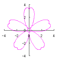
July 31, 2012


Fig.168  Petal as described
in the tiele
7.   Simulation in the case that the tip of the petals are pointed and also the base of the petals become thin
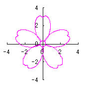
   We find that the the simulation of the flower as described in the title is obtained by plotting as in the orthogonal coordinates in the use of as an intermediate variable.   An example is shown in Fig.168 where .
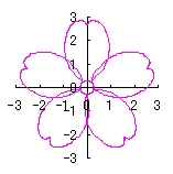
          .                      (96a)
          .                      (96b)
          .                 (96c)
          .                      (96d)
          .                      (96e)
          .                      (96f)
          .                      (96g)

   The C++ program for to calculate the numerical coordinates data of the curve shown in Fig.168 is given by Calculation program for Fig.168  &nbspflower_y1pre.
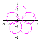
    number of the petals described above are placed around the center circle of radius .   The phase angle of such composed flower can be treated in the same manners as in [2.1 Additional II] and [2.2 Additional II] of Sec. 2, in [3.1.1 Additional II], [3.1.2 Additional II] and [3.2 Additional II] of Sec. 3 and in Sec. 6.1.2(ii).

          .                      (96h)
          .                      (96i)
          .                      (96j)
          .                      (96k)

   Calculating Eqs.(96j) and (96k), shape of flower may be drawn in the (x, y) coordinates.   Two examples such obtained are shown in Fig.169 and Fig.170 in the case of .


(If clicked,
an expanded line drawing appears.)
Fig.169 n=4, a=1, q1=1, q2=2, b=0.1,
d=8, e=0, k=1, l=0.2


(If clicked,
an expanded line drawing appears.)
Fig.170 n=4, a=1, q1=1, q2=2, b=0.1,
d=8, e=0, k=1, l=0.2


    The C++ program for to calculate the numerical coordinates data of the curve shown in Fig.169 and Fig.170 is given by Calculation program for Fig.169 and Fig.170  &nbspflower_y1.

June 17, 2013


_ returning to the page which opened just before with 'return' of browser _

or

_ returning to the HOME with the following button _


HOME

Updated: 2009.03.15, edited by N. Yamamoto.
Revised on July 2nd, 2012, July 09, 2012, July 14, 2012, July 18, 2012, July 22, 2012, July 25, 2012, July 29, 2012, July 31, 2012, Aug. 02, 2012, Sep. 12, 2012, Sep. 16, 2012, Sep. 23, 2012, Oct. 11, 2012, Oct. 17, 2012, Apr. 04, 2013, Apr. 12, 2013, May 09, 2013, May 15, 2013, June 17, 2013, Mar. 16, 2015, May 03, 2020, May 04, 2020, Jan. 23, 2021, May 08, 2021 and Mar. 20, 2022.